Table of contents
- 1. Understanding Bootstrap: The Motivation
- 2. Parametric Bootstrap: Not That Important
- 3. Non-parametric Bootstrap: It Is Important
- 4. Applications: Regression Coefficients
- 5. References
1. Understanding Bootstrap: The Motivation
Bootstrap is a powerful statistical tool used to quantify the uncertainty associated with a given statistic or estimator, such as the standard error or confidence interval.
Given that the population distribution is known, we can obtain the sampling distribution of a statistic/estimator by repeating the process of simulating N observations from the population K times, resulting in K realizations that approximate the sampling distribution.
- “The sampling distribution of a statistic is the distribution of all possible values of a sample statistic from all possible random samples drawn from the population.”
- Application in hypothesis testing: Assume H0 is true, then we could get the sampling distribution of the statistic. Then, we calculate the realized value of the statistic using the observed sample, then we can determine the p-value. If the p-value is very small, we can have confidence in rejecting H0.
However, in real-world scenarios, the population distribution is unknown. As a result, we cannot generate new samples from the original population. In such cases, we can sometimes rely on specific theorems that provide the sampling distributions for certain statistics or estimators, such as Central limited Theorem (CLT).
- CLT states that as the sample size gets larger, the distribution of the sample mean approximates a normal distribution, regardless of the population’s distribution.
- However, sampling distributions exist for any statistic that can be calculated from a sample, and in many cases, CLT cannot help. For example, the sample variance/sd will not follow a normal distribution. So? We might need to refer to other XXX theorems, or…
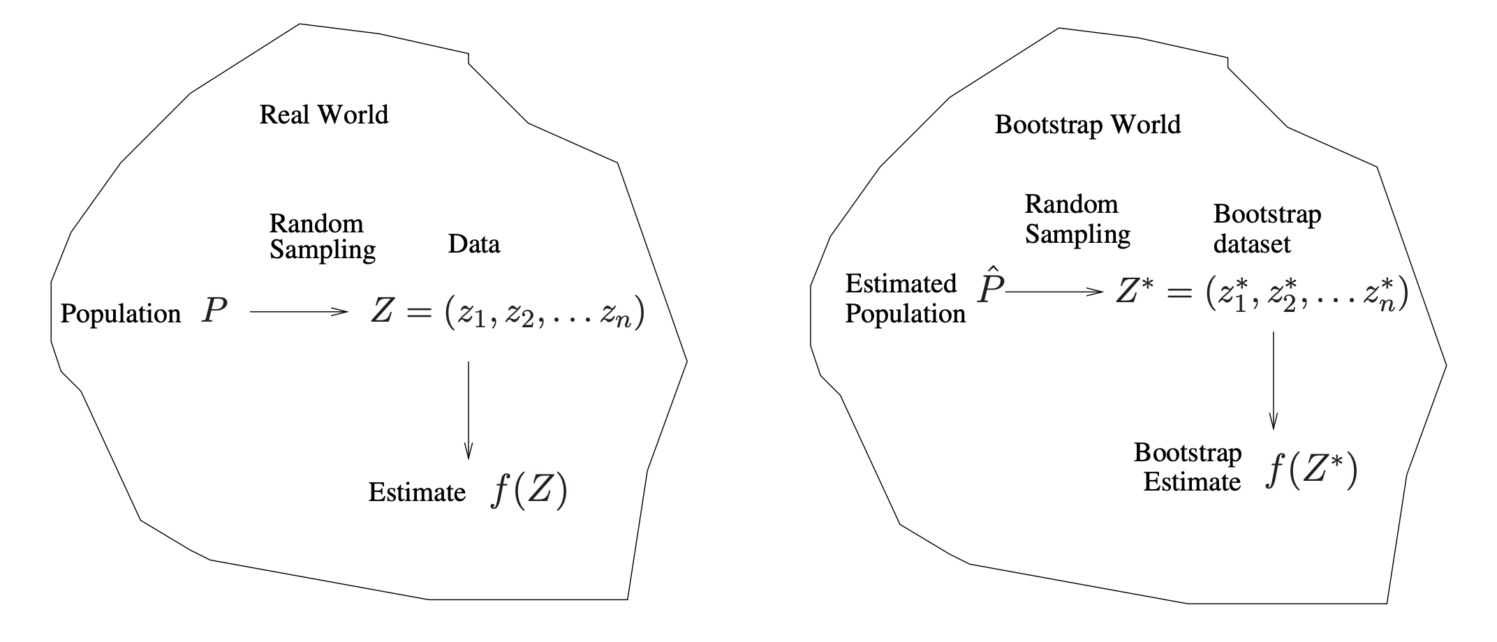
Even if we do not know the relevant theorem that indicates the sampling distribution, we can use simulation to approximate it >>> The bootstrap!
- First, make assumptions about the population >>> parametric/non-parametric.
- Then, repeatedly draw samples of a given size and record the statistic for each sample.
- Finally, get the sampling distribution.
2. Parametric Bootstrap: Not That Important
This approach assumes the population follows a specified parametric distribution.
- e.g., normal distribution >>> we make a so-called parametric assumption.
- Then, repeatedly draw samples from the assumed population…
3. Non-parametric Bootstrap: It Is Important
When we talk about “bootstrap,” we are usually referring to the non-parametric bootstrap. This is because the parametric bootstrap essentially involves repeatedly generating independent datasets from the (assumed) population. In contrast, the non-parametric bootstrap involves creating distinct datasets by repeatedly sampling the same number of observations from the original dataset with replacement.
- The NP bootstrap does not make any parametric assumptions about population distributions. The only non-parametric assumption: The sample is randomly drawn from the population and, therefore, can be representative of the population.
- We can generate more samples by duplicating our current observed sample multiple times through sampling with replacement. These “bootstrap samples” can serve as different samples drawn from the actual population, allowing us to derive the sampling distribution.
- As a result, some observations may appear more than once in a given bootstrap sample and some not at all.
- However, NP bootstrap works well only if the sample is reasonably large.

In more complex data situations, it is crucial to determine the appropriate method for generating bootstrap samples. Generally, when setting up the bootstrap and organizing the sampling process, you must identify which parts of the data are independent.
In addition to obtaining standard errors for an estimator, the bootstrap method also provides approximate confidence intervals for a population parameter, which called the Bootstrap Percentile Confidence Interval.
4. Applications: Regression Coefficients
4.1. Three Approaches
To derive the sampling distribution of the estimator in regression, we can use several bootstrap approaches:
- Empirical Bootstrap: Also known as the “paired bootstrap,” this method treats as one object. We then sample with replacement n times from these n objects to create a new bootstrap sample. For each bootstrap sample, we fit a linear regression.
- Residual Bootstrap: In this approach, we bootstrap the residuals and then regenerate Y. Using the bootstrap sample, we fit a linear regression as usual. We will delve into more detail about this process later.
- where
- Wild Bootstrap: The Wild Bootstrap is similar to the residual bootstrap, but it differs slightly in the way Y is regenerated.
- where
- For the i-th observation, the wild bootstrap uses only its own residual. In contrast, the residual bootstrap probably use the residuals from other observations.
4.2. Residual Bootstrap
God’s perspective (known distribution and parameter):
- Generate from a known distribution.
- Form for fixed and known .
- Compute .
- Repeat steps 1~3 many times.
- Estimate the sampling distribution of the estimated coefficients by the empirical distribution of the estimated coefficients from the simulated data sets.
Bootstrap’s perspective (unknown distribution and parameter):
- Generate by sampling with replacement from .
- i.e., resample the residuals, whose mean is exactly 0.
- Regenerate for fixed X and known .
- Compute from .
- i.e., bootstrap estimator .
- Repeat steps 1~3 many times.
- Estimate the sampling distribution of the estimated coefficients using the bootstrap distribution of the estimated coefficients from the bootstrapped data sets.
5. References
- Chen, Y. (2017). Bootstrap regression. https://faculty.washington.edu/yenchic/17Sp_403/Lec6-bootstrap_reg.pdf
- Freedman, D. A. (2009). Chapter 8. In Statistical models: Theory and practice (2nd ed., pp. 155-175). Cambridge University Press.
- Lin, H.-T. (2020). Machine Learning Handout. National Taiwan University. Retrieved from https://www.csie.ntu.edu.tw/~htlin/course/ml20fall/doc/210_handout.pdf
- Miles Chen. (2021, March 4). Stats 102A Lesson 9-2 Bootstrap Hypothesis Tests [Video]. YouTube. https://www.youtube.com/watch?v=s7do_F9LV-w&list=PLKR7271tMEmgsp83ZJPMr96xd-8fPq3p1&index=25
- Stanford Online. (2022, October 8). Statistical Learning: 5.4 The Bootstrap [Video]. YouTube. https://www.youtube.com/watch?v=h_LweqiIotE
- Stanford Online. (2022, October 8). Statistical Learning: 5.5 More on the Bootstrap [Video]. YouTube. https://www.youtube.com/watch?v=OKREmw6YP64
- StatQuest with Josh Starmer. (2021, July 6). Bootstrapping Main Ideas!!! [Video]. YouTube. https://www.youtube.com/watch?v=Xz0x-8-cgaQ