Table of contents
- What is the chi-square test?
- One variable - Distribution test
- Two variables - Independence test
- Chi-squared test for trend
- References
What is the chi-square test?
The chi-square test(卡方检验), also known as the test of goodness of fit(拟合优度检验), is used to determine whether a set of observed data conforms to a particular theoretical distribution.
More specifically, it can test whether a categorical variable follows a particular distribution (distribution test) or whether two categorical variables are independent (independence test).
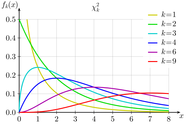
Since the statistic used in the tests follow a chi-square distribution when the null hypothesis is true, it is called a chi-square test.

The variables involved in chi-square tests are typically categorical. However, when dealing with continuous variables, such as testing the “H0: data comes from a normal distribution,” the data can be discretized first and processed similarly to categorical variables.
One variable - Distribution test
Use the sample to test the hypothesis:
Test statistic:
represents the observed frequency of category i, while represents the expected frequency of category i under the H0. Hence, the larger the statistic Z, the easier it is to reject H0.
Furthermore, when H0 is true and the sample size n is large enough, Z follows a chi-square distribution with k-1 degrees of freedom. Based on that, we can calculate the p-value or threshold and make a conclusion accordingly.
Two variables - Independence test
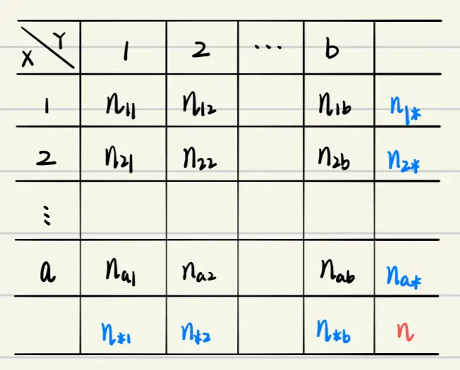
There are two categorical variables. Their ranges are:
Our sample is shown in the following contingency table(列联表):

In this scenario, the null hypothesis is (i.e. no relationship):
or equivalently represented as:
First, estimate the marginal distributions:
Test statistic:
When H0 is true and the sample size n is large enough, Z follows a chi-square distribution with (a-1)(b-1) degrees of freedom. Based on that, we can calculate the p-value or threshold and make a conclusion accordingly.
Chi-squared test for trend
In both of the cases mentioned above, we haven’t specified whether the categorical variables involved are nominal(名义变量) or ordinal(定序变量). When dealing with ordinal variables, using the chi-square test in aforementioned ways (also referred to as “Pearson’s chi-squared tests”) fails to leverage the information provided by their ordering:
In spite of its usefulness, there are conditions under which the use of Pearson’s chi-square, although appropriate, is not the optimum procedure. Such a situation occurs when the categories forming a table have a natural ordering.
There are several other tests that take into account the ordering information when dealing with ordinal variables, such as the Cochran–Armitage test for trend and the Mantel-Haenszel linear-by-linear association test.
- Cochran–Armitage test → binary × ordinal: whether the positivity rate increases or decreases with the increasing levels of the ordinal variable (i.e. linear trend in the proportions). Here is the R code and demo.
library(DescTools)→CochranArmitageTest
- Mantel-Haenszel test → ordinal × ordinal: whether there is a linear correlation between the two ordinal variables (i.e. linear relationship). It is enabled by default in SPSS.
- source file →
MH.testorMH.test.mid library(DescTools)→MHChisqTest
- source file →
References
- 陈希孺(2009):《概率论与数理统计》,第5.3节
- Agresti, A. (2019). An introduction to categorical data analysis. Wiley.
- Detailed intro to chi-square test from a medical statistics perspective
- Chi-Squared Test for Association in SPSS
- Chi-Square - Sociology 3112 - The University of utah
- About the use and misuse of chi-square
- Yates’s correction for continuity - Wikipedia