Method | A Crash Course For Bayesian Inference

This is the final presentation for {SG8001: Teaching Students: First Steps}.

1. After This Crash Course, You Will Be Able To:
2. How to Infer? Frequentist vs. Bayesian Perspective
3. Three Components in a Bayesian Pipeline
4. Toy Example: Biased Coin
5. Take-Home Notes
6. Get your hands dirty

1. After This Crash Course, You Will Be Able To:

Understand the fundamental differences between frequentist and Bayesian philosophies, and explain the advantages of the Bayesian approach.
Identify the three key components of Bayesian inference and describe the general workflow for conducting simple Bayesian analysis.
Apply the Bayesian approach to solve basic inference problems, including the selection and interpretation of different priors.

2. How to Infer? Frequentist vs. Bayesian Perspective

Statistical inference is a process of using a random sample to draw conclusions about the unknown characteristics of an underlying population.

When you’ve used methods like Maximum Likelihood Estimation (MLE) to generate point estimates, build confidence intervals, or conduct hypothesis tests using p-values, you’ve been working within the frequentist framework.

However, this approach has some limitations. For instance:

It only uses the observed data, even when it would be more beneficial to account for the entire data-generating process, not just the sample at hand.
It disregards any prior knowledge you may have, even if that information could enhance the accuracy of your inferences.

Bayesian inference, on the other hand, takes a different approach to addressing these challenges by offering a more flexible philosophical framework:

It treats all probabilities as subjective, reflecting uncertainty due to insufficient information. This allows us to assign probabilities to model parameters, giving a theoretical basis for capturing the full data-generating process.
It allows us to formally incorporate prior knowledge alongside the observed data. By doing so, Bayesian methods often return more reliable results, especially in situations with small sample sizes.

3. Three Components in a Bayesian Pipeline

Bayesian inference is essentially about using observed data to update prior knowledge about the population, resulting in what is called the posterior. You can make further inferences about the population using this updated knowledge, which incorporates both the current data and your original beliefs. The three core components in this updating process are:

Likelihood p(D|θ): The likelihood refers to the probability of the data D, given the population parameter θ. This definition is the same as in the frequentist approach.
Prior p(θ): The prior is the subjective probability of the parameter θ. It is assigned to θ at the very beginning, reflecting your initial belief about what the population might be. This is one of the key differences between frequentist and Bayesian approaches: for the former, the parameter is unknown but fixed, while for the latter, the parameter is treated as a random variable (in the mind of the person) so that we can give it a probability distribution.
Posterior p(θ|D): The posterior represents our updated belief about the distribution of θ after observing the data D. This means that we incorporate the information in the data into our original belief (the prior), resulting in what we call the posterior.

Using Bayes’ rule, we can link these three components together to understand how to update from prior to posterior:

p(\theta|D) = \frac{p(D|\theta)p(\theta)}{p(D)} = \frac{p(D|\theta)p(\theta)}{\sum_{\theta} p(D|\theta)p(\theta)}

The denominator is the normalization factor, often called evidence, or the average probability of the data over the prior. Once we plug in the observed data and integrate (or sum) over θ, it becomes a constant number. Hence, when performing tasks like MAP, we can effectively ignore the denominator and only maximize the numerator (although we often do not recommend using MAP, as it wastes a lot of the information brought by the posterior):

p(\theta|D) \propto p(D|\theta)p(\theta)

Next, we will dive into a toy example to illustrate this Bayesian pipeline.

4. Toy Example: Biased Coin

Consider a biased coin with an unknown probability θ of landing heads (H). You toss the coin five times and observe the following sequence: HTHHH (where T represents tails). Your task is to estimate θ based on this data. Let’s solve this problem using Bayesian inference.

First, we can write the likelihood function:

p(D|\theta) = \theta^4 (1-\theta)

Next, we need to choose a prior distribution before proceeding.

1) Uniform(0,1) as Prior

This prior indicates that we have no prior knowledge about the coin’s bias, meaning every value of θ between 0 and 1 is equally likely. This is known as an uninformative prior in this context. The probability density function is:

p(\theta) = 1

the posterior distribution is proportional to the likelihood times the prior:

p(\theta|D) \propto p(D|\theta)p(\theta) = \theta^4 (1-\theta)

To find the Maximum A Posteriori (MAP) estimate, we maximize the posterior:

\argmax_{\theta}\ p(\theta|D) = \argmax_{\theta}\ \theta^4 (1-\theta) = 0.8

This result is identical to the Maximum Likelihood Estimate (MLE) in the frequentist approach.

2) Beta(2,2) as Prior

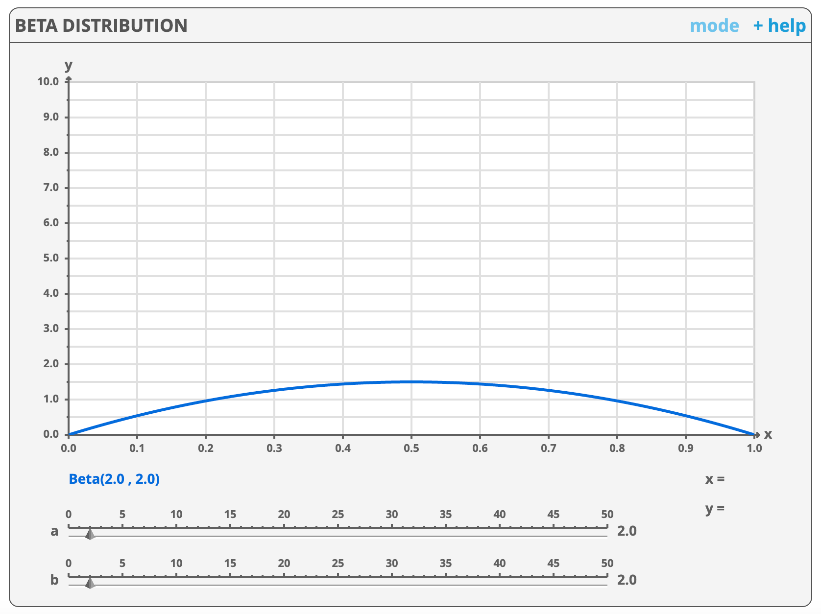
Now, let’s assume a Beta(2,2) prior, reflecting our prior belief that the probability of heads is centered around 0.5, but with some uncertainty. This prior is informative, encoding a modest amount of initial belief before observing any data. The prior distribution is:

p(\theta) = \text{Beta}(\theta;2,2)

Thus, the posterior is:

p(\theta|D) \propto \theta^4 (1-\theta) \times \text{Beta}(\theta;2,2) = \cdots = \text{Beta}(\theta;6,3)

Maximizing the posterior gives us the MAP estimate:

\argmax_{\theta}\ p(\theta|D) = \frac{5}{7} \approx 0.714

Comparing this with the previous estimate, we can see that θ=0.714 is pulled slightly closer to 0.5, reflecting the influence of the prior belief that θ is likely around 0.5.

3) Beta(20,20) as Prior

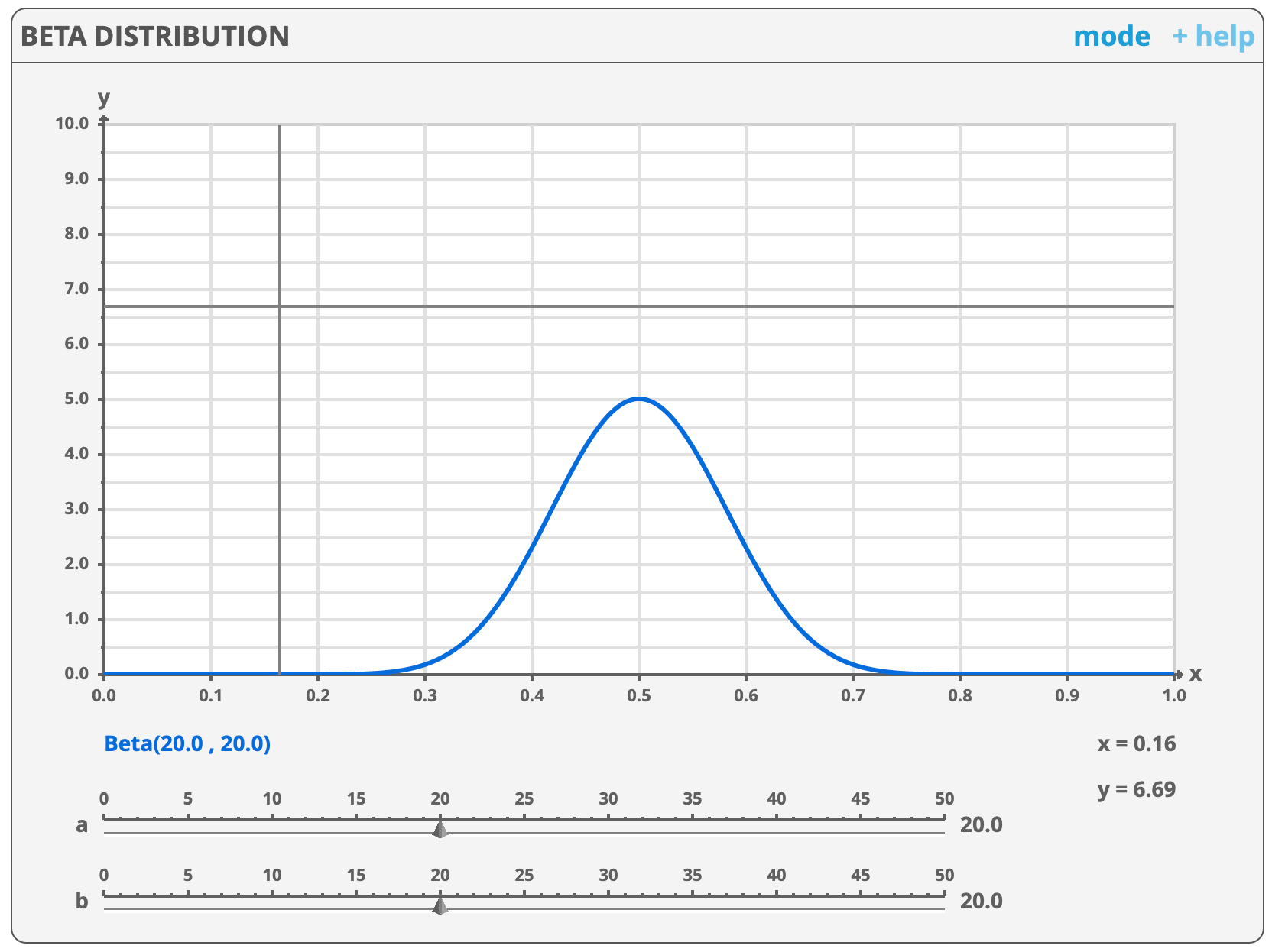
In this case, we use a Beta(20,20) prior, which indicates even greater confidence that the coin is balanced before observing the sequence HTHHH. After incorporating the observed data, the posterior becomes Beta(24,21). Using MAP, we estimate θ as (24-1)/(24+21-2)=23/43=0.535.

This estimate is significantly lower than the estimate from the Beta(2,2) prior, bringing it closer to 0.5, which reflects the stronger influence of our more confident prior belief.

5. Take-Home Notes

Compared to the frequentist approach, the Bayesian approach treats probability as a subjective belief, focusing on modeling the underlying data-generating process and incorporating prior knowledge into the model.
Bayesian inference uses observed data to update prior knowledge about the population, resulting in the posterior distribution.
According to Bayes’ rule, the posterior is proportional to the product of the likelihood and the prior.
The same data analyzed with different priors can lead to different results. When you have little prior information, use an uninformative prior; otherwise, you can express your initial belief through an informative prior.

6. Get your hands dirty

Suppose you‘re trying to estimate the true value of a parameter $\mu$ , which represents the mean of a normal population with a known variance $\sigma^2=1$ . You have a sample of observed data consisting of independent measurements: $x = [2.1, 1.9, 2.2, 2.0, 1.8]$ . Try to use different normal priors and perform MAP estimations. Then, compare the results with the MLE result.