Although we have derived a beautiful result (i.e. high accuracy) from gradient boosting algorithms, we still want to know how the deep learning model performs in this task. Because there is little information about time series in this data set, we choose to use a simple feed-forward neural network as our deep learning model.
Table of contents
- 1. Toolkit: PyTorch
- 2. Data preprocessing
- 3. Network structure
- 4. Hyperparameter tuning
- 5. Retrain & Test
- 6. Explainable deep learning model
- 7. Discussion
1. Toolkit: PyTorch

PyTorch is an open source machine learning library and is widely used in deep learning scenarios for its flexibility. PyTorch uses dynamic computational graphs rather than static graphs, which can be regarded as the mean difference between it and other deep learning frameworks. To get more information on PyTorch, click here.
2. Data preprocessing
Drop some features: As we did before, two features (“reservation_status_date” & “reservation_status”) are dropped for avoidance of leakage. In addition, we drop the feature “arrival_date_year” because we will use future information to predict future cancellation behavior.
One-hot encoding: One-hot encoder is used to convert categorical data into integer data. Since there are many categories under “company” and “agent”, data’s dimension increases to 1025 after the one-hot encoding.
Validation set: We use 20% data in train.csv as our validation data.
3. Network structure
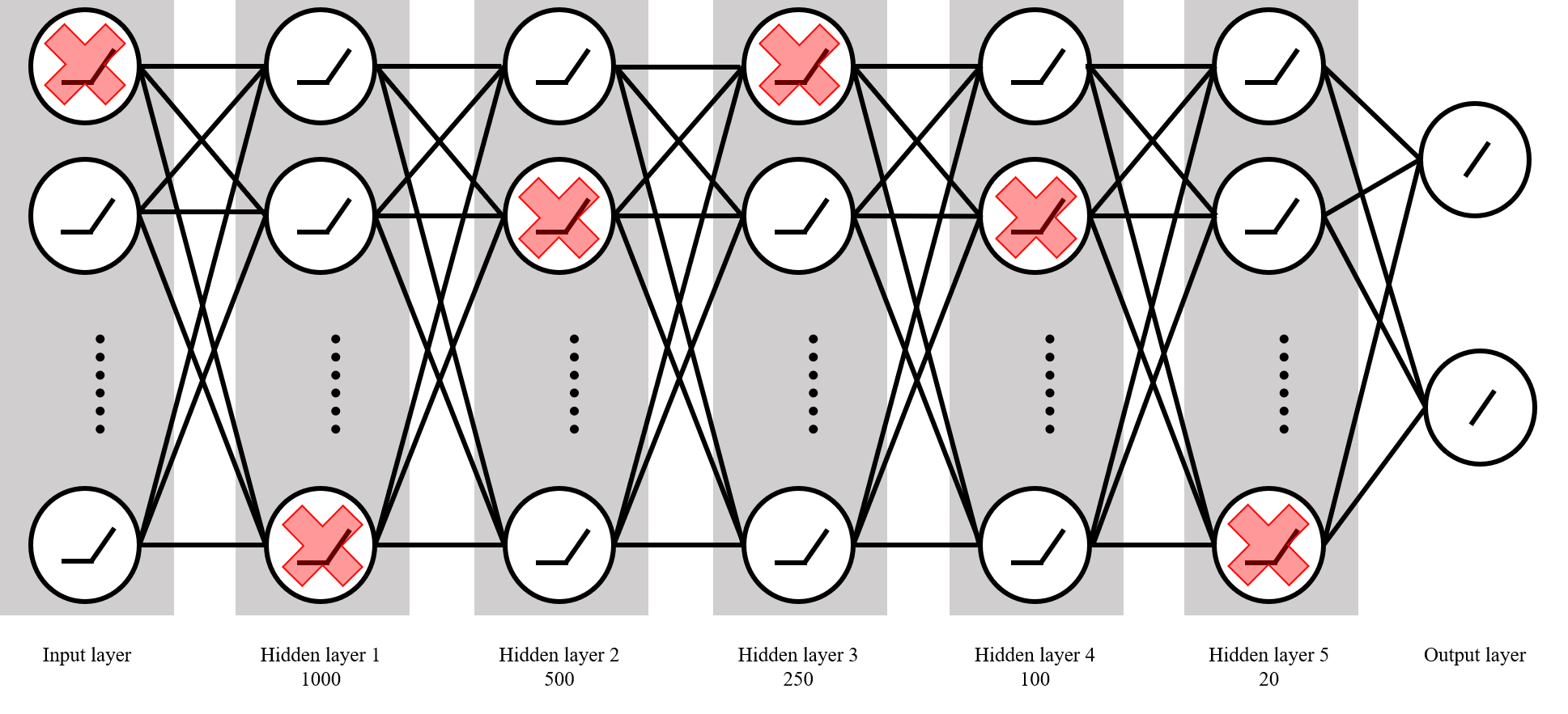
- Input→1000→500→250→100→20→2
- Dropout after doing batch normalization
- Choose Sigmoid/Tanh/ReLU as activation function
4. Hyperparameter tuning
It is a binary classification task, so we use cross-entropy as our loss function and apply early stopping to avoid over-fitting. Because we use dropout as a tool of regularization, we need to determine the dropout rate dr. We use Adam as adaptive learning rate method and fix beta_1 and beta_2 by using their default values, but we still need to determine the learning rate lr. At last, we want to compare the average performance of three kinds of activation function (sigmoid, Tanh, ReLU). Hence, there are three kinds of parameters that need to be tuned:
- learning rate lr for Adam: [0.005, 0.05]
- dropout rate dr: [0.2, 0.8]
- activation function: sigmoid, tanh, ReLU
We use random search rather than grid search for hyperparameter tuning —— Randomly select 120 parameter combinations. The result is as follows:
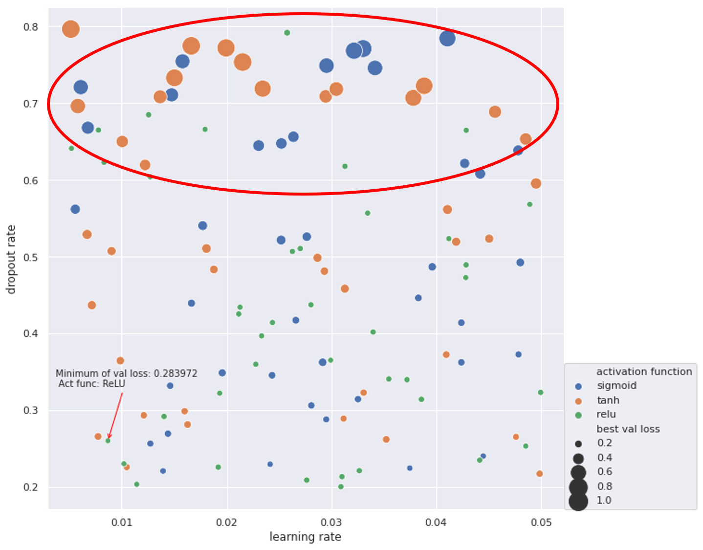
The best parameters among these 120 combinations are:
- learning rate: 0.00867688
- dropout rate: 0.260069
- activation function: ReLU
The corresponding validation loss is 0.283972. The validation accuracy is 0.870927. From the scatterplot, we can see that ReLU is a better choice for activation function because of its stableness. When dropout rate is high (0.6~0.8), using sigmoid or tanh as activation function will get bad results (loss approx 1.0). However, ReLU can still provide a small loss and high accuracy in that region.
5. Retrain & Test
At last, we use the hyperparameters from the last step and retrain the model on the whole training data (original training set + validation set). The learning process:
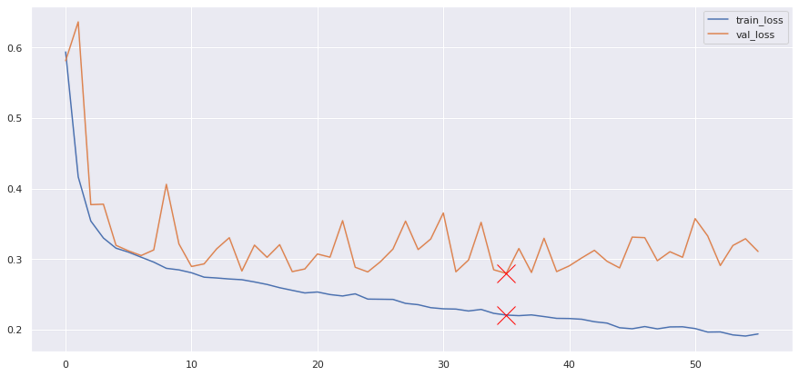
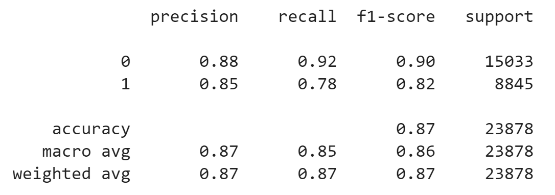
The test loss is about 0.280 and test accuracy is about 0.875. Other performance metrics on test set:
6. Explainable deep learning model
At last, we want to make this deep learning model explainable in some sense. So we try to apply LIME (Local Interpretable Model-agnostic Explanations) on the model we trained above in order to get some hints from the local explanation.
- First, we notice that DL model predicts the 21st test instance as [label 1] with probability distribution [0.00001, 0.99999]. We choose this data point as our ”local point“.
- Second, we sample 5000 instances nearby. In particular, we fix the value of categorical variables and only do sampling in terms of numerical variables for convenience.
- Use DL model to predict the labels of these 5000 sample. After that ,we get 5000 new ”training data“.
- We choose logisitic regression as the simple model to explain the DL model locally —— Train the LR model on 5000 new “training data” in order to mimic the DL model’s behavior locally. The accuracy is 98.86%.
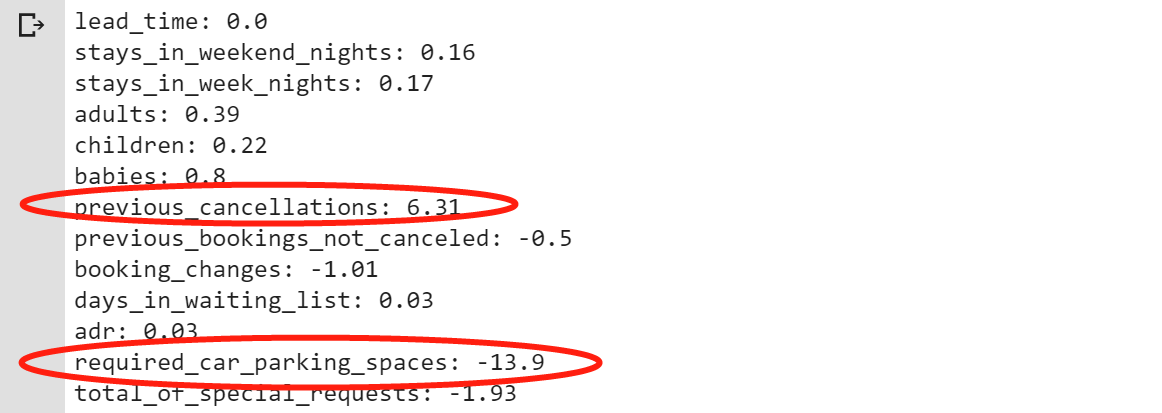
- Finally, we get the coefficients before the numerical variables. It is worth noting that the coefficient before “previous_cancellations” is +6.31 and the coefficient before “required_car_parking_spaces” is -13.9. This result shows the judgment logic of the DL model: people who have cancelled the order before have a higher probability of canceling this order and people who reserved parking spaces are less likely to cancel this order.
7. Discussion
In this task, it seems that deep learning model can not beat the gradient boosting method. There are some possible reasons. First, we know that deep learning model is more powerful when dealing with unstructured data such as images and text by extracting meaningful representations. However, in this task, all data is structured. Second, in such context, deep learning models need to adjust more parameters in order to get a better result. Among all the hyperparameters, the network structure is very important. However, due to insufficient computing power, we fixed the network structure in advance. Therefore, we may be trapped in a bad network structure at the beginning.