Network | Node Embeddings

Source: Stanford CS224W: Node Embeddings & Lecture Video

Table of contents

• 1. Motivation: Graph Representation Learning
• 2. Core Components of Node Embeddings
• 3. Random Walk Approach for Node Embeddings
  • 3.1 Problem Statement
  • 3.2 Optimization Problem
  • 3.3 Random Walk Strategy

1. Motivation: Graph Representation Learning

The traditional approach to machine learning for graphs involves extracting features at the node, edge, or graph level from the graph structure and then using these features in supervised learning to predict the graph’s label:

Graph representation learning, on the other hand, transforms the feature engineering process from a manual effort into an automated one, allowing features to be automatically extracted from the graph:

One approach to graph representation learning is node embeddings, which map the nodes of a graph into a (low-dimensional) embedding space using a learned function $f$:

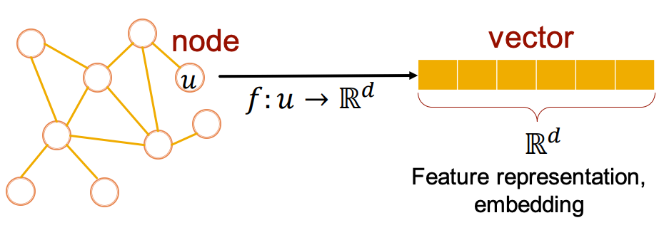
The function $f$ must satisfy some intuitive conditions. For example, if two nodes are close in the embedding space, it implies they are also similar in the network. In other words, function $f$ should effectively encode the network’s structural information.

It’s important to note that network embeddings encompass a broader scope compared to node embeddings. The former includes learning low-dimensional representations for nodes, edges, or entire graphs, ensuring that the graph’s structural and relational properties are preserved.

2. Core Components of Node Embeddings

We denote the graph by G, with its corresponding adjacency matrix denoted by A, and the node set denoted by V. The goal of node embeddings is to encode nodes so that similarity in the embedding space (e.g., dot product) approximates similarity in the graph:

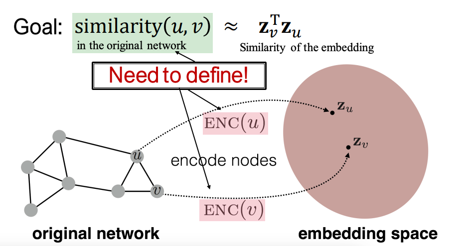
There are four key components in this process:

1. Encoder
   • $\text{ENC}(v) = \mathbf{z}_v$ (a d-dimensional embedding)
   • Essentially, this step provides a unique embedding vector for each node, aligning them into a matrix $Z \in R^{d \times |V|}$
   • Methods: DeepWalk, node2vec, GNN, etc.
2. Node similarity function
   • A measure of similarity in the original graph/network: are linked? share neighbors? have similar “structural roles”?
   • One approach: similarity based on “random walks”
3. Decoder
   • Use the embeddings $\mathbf{z}_v$ and $\mathbf{z}_u$ to calculate the similarity score $\text{DEC}(\mathbf{z}^T_v \mathbf{z}_u)$
   • For example, the decoder can simply be y=x, making the similarity score a straightforward dot product.
4. Optimization
   • Optimize the parameters of the encoder so that $\text{similarity}(u,v) \approx \mathbf{z}^T_v \mathbf{z}_u$

3. Random Walk Approach for Node Embeddings

3.1 Problem Statement

Random walk: Given a graph and a starting point, a neighbor is selected at random. At last, the (random) sequence of points visited this way is a “random walk on the graph”. Rules can be set for this process, referred to as the “random walk strategy R”.

Node similarity based on random walk approach: node u and node v are similar if they have high probability that u and v co-occur on a random walk over the graph. Alternatively, given a node u, we define a set of nodes $N_R(u)$ which denotes the neighborhood of u obtained by some random walk strategy R. These nodes are considered similar to node u.

Now, we try to frame the problem as an optimization problem: our goal is to learn node embeddings such that nodes that are close in the graph are also close in the embedding space:

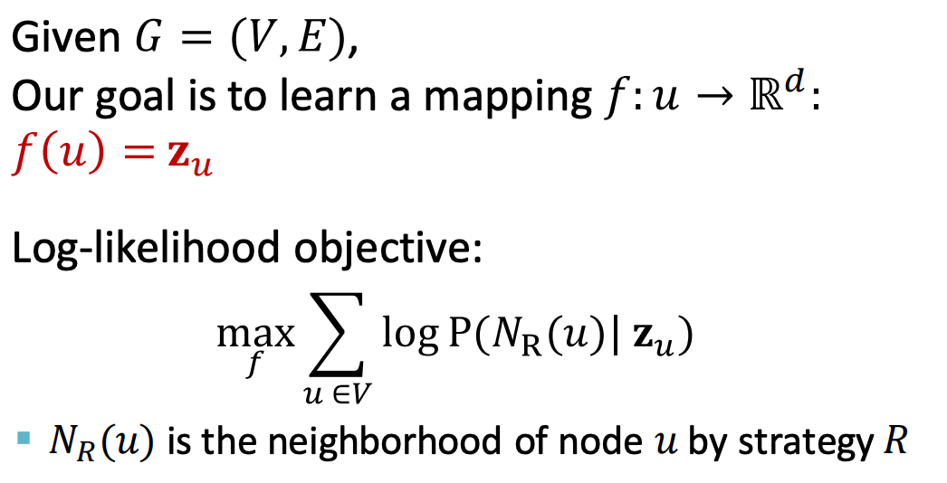
In the objective function, $P(N_R(u)|\mathbf{z}_u)$ represents the predicted probability that the sequence generated by a random walk starting from node u is exactly $N_R(u)$. Next, we will parameterize this quantity. Before that, two notable advantages of the random walk approach are:

1. It allows for a flexible definition of node similarity within a network, incorporating both local and higher-order neighborhood information.
2. It eliminates the need to consider all node pairs during training; instead, only pairs that co-occur on random walks need to be evaluated.

3.2 Optimization Problem

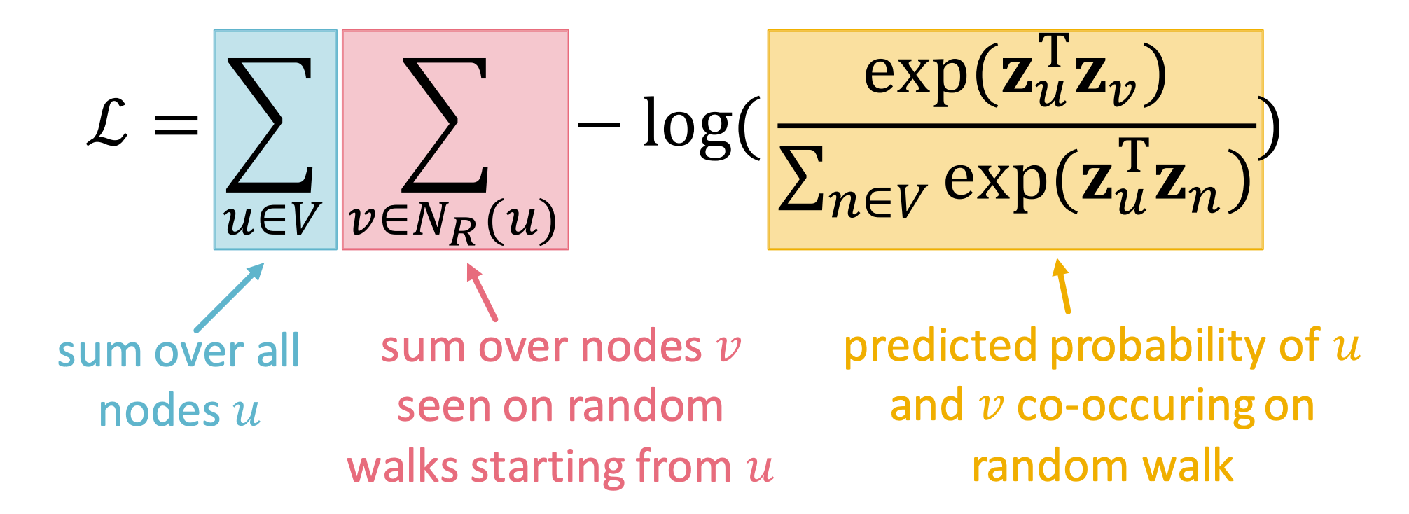
We proceed to further transform the objective function:

1. Convert the maximization problem into a minimization problem.
2. Expand the log probability $\log P(N_R(u)|\mathbf{z}_u)$ as $\sum_{v\in N_R(u)} \log P(v|\mathbf{z}_u)$.
3. Parameterize $P(v|\mathbf{z}_u)$ using the softmax function over all nodes in the graph.

However, there is a dilemma: solving this optimization problem is computationally expensive, with a complexity of $O(|V|^2)$! This is primarily because, for a given node u, computing $P(v|\mathbf{z}_u)$ requires traversing all nodes in the graph to perform normalization.

Can we limit this process to a subset of nodes instead of all nodes? Yes, by using negative sampling: instead of normalizing with respect to all nodes, we normalize using only k randomly chosen “negative samples”:

Here are some practical guidelines without going into details: 1) How to sample k negative nodes? The sampling distribution is proportional to the degree of each node. 2) Choosing k: In practice, k typically ranges from 5 to 20.

Finally, SGD is commonly used to solve this optimization problem.

3.3 Random Walk Strategy

How should we perform a random walk? It depends on the chosen random walk strategy R:

• Using different strategies R, the resulting neighborhood $N_R(u)$ for the same node can vary.
• The simplest approach involves fixed-length, unbiased random walks.
• Alternatively, biased random walks can be used to balance between a local and global view of the network - Two classic strategies (BFS vs. DFS) are commonly used to define the neighborhood $N_R(u)$ for a given node u:

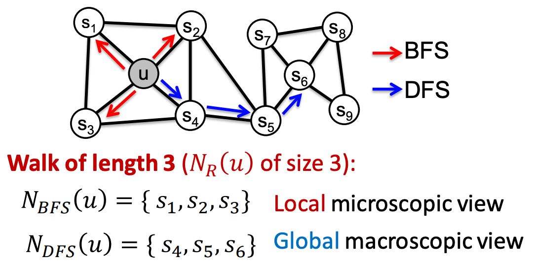
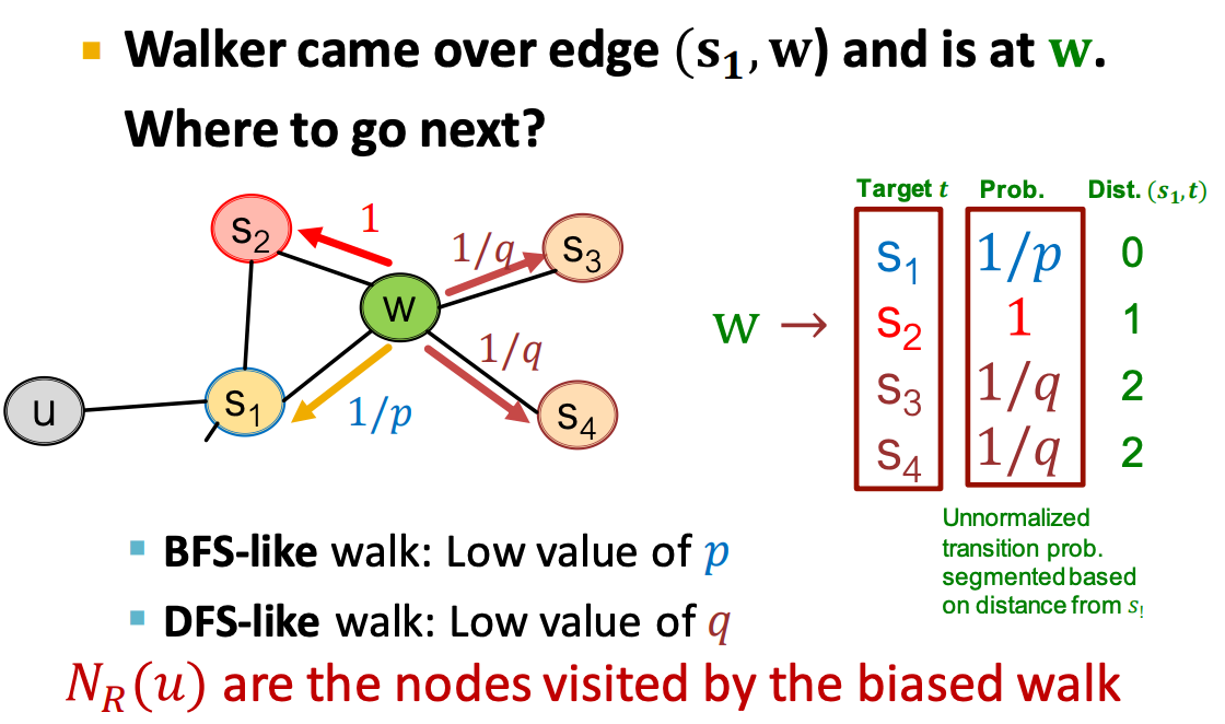
These two strategies above can be combined into a biased fixed-length random walk characterized by two parameters: 1) Return parameter p: Controls the likelihood of returning to the previous node. 2) In-out parameter q: Balances between BFS (i.e., moving to a neighboring node) and DFS (i.e., moving to a deeper node):

Finally, the node2vec algorithm:

• Compute random walk probabilities.
• Simulate $r$ random walks of length $l$ starting from each node $u$.
• Optimize the node2vec objective using SGD.