Table of contents
- 1. The Basic
- 2. Application
- 3. Related Distribution: The Binomial
- 4. Poisson Regression
- 5. Poisson Regression with Offset
- 6. Example: Age-Grouped Cancer Incidence in Danish Cities
- 7. References
1. The Basic
The pmf of a Poisson random variable :
where called the “rate” parameter. This pmf can be easily verified as valid by using the fact that is the Taylor expansion of at 0. Also, we have:
2. Application
The Poisson distribution is often used to count the number of “successes” in scenarios involving a large number of trials, each with a small probability of success. For example,
- The number of emails received in an hour
- The number of earthquakes happened in a year
- The number of accidents occurring at a intersection during a period of time.
“The Poisson Approximation”: Event with , is large and ’s are all small; These events are independent or weakly dependent >>> Then, the number of events that occur is approximately a Poisson with .
3. Related Distribution: The Binomial
Let . As and such that remains constant (i.e., their rates of convergence are similar), the pmf of converges to the pmf of a Poisson distribution with parameter .
Summary: Binominal can converge to a Poisson in a certain way.
4. Poisson Regression
Poisson regression should be used when DV is a count variable, such as the number of times an event occurs in a given time period. Model specification:
- Model estimation: MLE
- Model explanation:
- intercept : When all IVs are 0, the mean of DV is .
- slope : When all other IVs are held constant, increasing by one will multiplies the mean of DV by .
5. Poisson Regression with Offset
Special case: when ’s represent the counts within the different time interval.
- For instance, represents the number of phone calls within 1 hour, represents the number of phone calls within 3 hours…
In this case, the data are like , instead of the original . We can still use the Poisson model with a slight modification as follows:
Here, represents the count per unit length of time and represents the number of time units. Then, we perform the following transformation:
Let , and then we can treat it as a “standard Poisson regression + adjusted systematic linkage.” Here, is referred to as the offset.
6. Example: Age-Grouped Cancer Incidence in Danish Cities
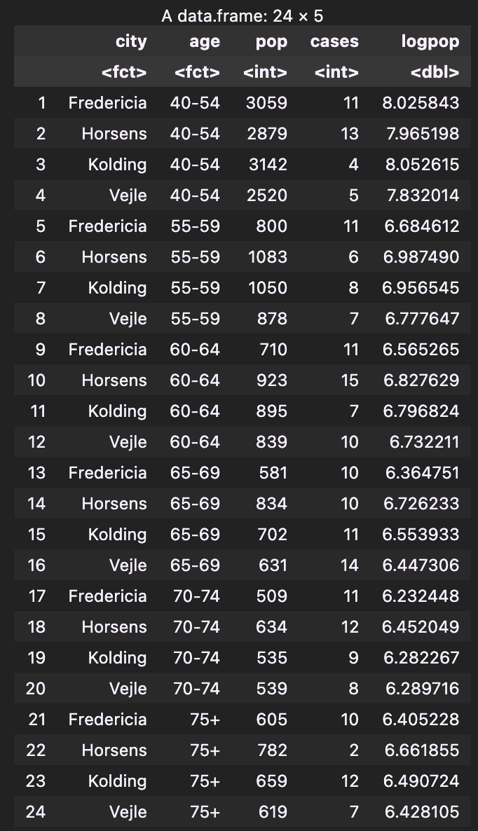
The eba1977 dataset from the ISwR package contains counts of incident lung cancer cases and population size in four neighbouring Danish cities by age group:

In this dataset, “pop” (i.e. population) is an attribute regarding to interval. Thus, we should use the Poisson model with offset. In this case, represents the “#cancer cases/per person”, which is exactly the probability of developing cancer.
## Import data
data(eba1977)
cancer.data = eba1977

## Add the offset column
logpop = log(cancer.data[ ,3])
new.cancer.data = cbind(cancer.data, logpop)

## GLM model
model = glm(cases ~ city + age+ offset(logpop),
            family = poisson(link = "log"), data = new.cancer.data)
summary(model)
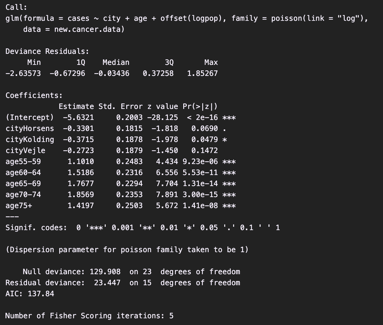
The summary report:

Interpretation of some coefficients:
Intercept = -5.63 (***): The probability of developing cancer for a person aging 40-54 and living in Fredericia is .cityKolding = -0.37 (*): For individuals in the same age group, the probability of developing cancer in the city of Kolding is exp(-0.37)=0.69 times that in the city of Fredericia.age75+ = 1.42 (***): For individuals living in the same city, the probability of developing cancer for those aged 75+ is exp(1.42)=4.14 times that for those aged 40–54.
7. References
- Harvard University. (2013, April 30). Lecture 11: The Poisson distribution | Statistics 110 [Video]. YouTube. https://www.youtube.com/watch?v=TD1N4hxqMzY&list=PL2SOU6wwxB0uwwH80KTQ6ht66KWxbzTIo&index=11
- NYCU OCW. (2016, October 28). Lec 31 Poisson regression and log-linear model [Video]. YouTube. https://www.youtube.com/watch?v=eQejmHDjd4Y&list=PLj6E8qlqmkFu0cY9PfwoFq6SbuZ-M28JE&index=31