Summary
| Type | Regression Formula | Y | X | M |
|---|---|---|---|---|
| One-way ANOVA | Y ~ X | scalar | discrete | / |
| Two-way ANOVA (× replication) | Y ~ X + M | scalar | discrete | discrete |
| Two-way ANOVA (√ replication) | Y ~ X + M + X * M | scalar | discrete | discrete |
| ANCOVA | Y ~ X + M + X * M | scalar | discrete | continuous |
| MANOVA | Y ~ X | vector | discrete | / |
Table of contents
1. One-way ANOVA
Y ~ X
1.1 Experiment design
In a location that has never grown wheat before, wheat cultivation begins with selecting varieties (品种) through field experiments. There are varieties and experimental fields - each variety occupies fields, which allows for the estimation of random errors.
Once the number of fields for each variety is determined, the fields are allocated using a randomization (随机化) method - This prevents the case that a variety is assigned to a particularly fertile field, leading to higher yields unrelated to the variety’s qualities.
The objective is to compare the yield differences among the various wheat varieties and identify the most suitable variety for cultivation in the region. Here,
- “variety (品种)” is referred to as a “factor (因素)”
- “each specific variety (具体的某个品种)” = “a specific level (水平) of that factor”
- Thus, this experiment is called a single-factor experiment with k levels (单因素k水平).
1.2 Model specification
Let denote the j-th observation of the i-th level:
- variety 1: , , …,
- variety 2: , , , …,
- …
Our model:
- : mean of the level i
- : random error with mean 0 and fixed variance
Our question / null hypothesis:
Assumptions:
- Observations within each level/group must be independent and identically distributed.
- The response variable should be normally distributed for each group.
- All groups should have the same variance.
1.3 Theoretical analysis
Why vary?
- Variation source 1: ,即不同组之间本身水平就有差异。
- Variation source 2: ,即随机误差一直存在。
- An intuitive idea is to decompose the total variation into these two parts, to see if the source of variation 1 is sufficiently large.
Total variation (Y_bar = average across all individuals):
Variation due to random error (i.e. 组内变异):
Variation due to different level (i.e. 组间变异):
1.4 Full test: a1=a2=…=ak?
When the proportion of SSA in the SS is higher, it is easier to reject our previously stated H0. Therefore, the test statistic we choose is:
When the random error term follow a normal distribution and H0 is true, it follows that:
Set the test level at . Accept H0 when:
, otherwise reject H0. Note, if the test result is significant (reject H0), then there is reason to believe that a1~ak are not all the same — but this does not necessarily mean that none of them are the same.
1.5 Partial test: a_u=a_v?
We can test whether by calculating the confidence interval (CI) for .
Hence, the point estimate of , , follows:
Then we have:
MSE is an unbiased estimate of . Substitute for :
We can construct a CI for with a confidence coefficient of . If 0 is not within this CI, then it indicates that there is indeed a significant difference between and .
[Warning! Inflation of type I error] For just a single pair and , the probability that the CI contains the parameter is . However, when constructing confidence intervals for multiple pairs, the probability that all intervals include their parameters decreases to . For example, if and , the probability that all 10 intervals contain their parameters is only . Therefore, for pairwise comparisons, alternative methods such as the Tukey–Cramer Method should be considered, instead of direct pair comparisons.
1.6 Connection with regression
Single-factor (k levels) ANOVA is equivalent to a linear regression with one categorical variable that can take k values. Thus, it can be transformed into k-1 dummy variables included in the linear regression model.
2. Two-way ANOVA
2.1 Without replication
Y ~ X + M
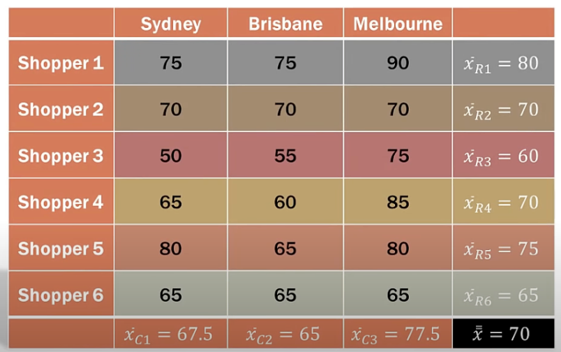
In this case, we have two factors: factor A has levels and factor B has levels. The total number of unique combinations of these factors is . Unlike the previous setting where multiple experiments () are conducted for each level of a single factor, here we conduct only one experiment for each combination of Factor A and Factor B levels.
Our model:
- : total average
- : increment due to level i of factor A
- : increment due to level j of factor B
Our null hypotheses:
Variance decomposition:
Total variation is caused by variation among levels in factor A, variation among levels in factor B, and random error. The test statistics are similar to those in the single-factor setting: the larger the , the more probable it is to reject the null hypothesis that factor A does not have a significant impact on DV.
Why we do two-way ANOVA without replication? Introducing a new factor (i.e. independent variable) can further decompose the SS, resulting in a smaller SSE; thus, group differences that were not detectable in one-way ANOVA might be detected here.
2.2 With replication
Y ~ X + M + X*M
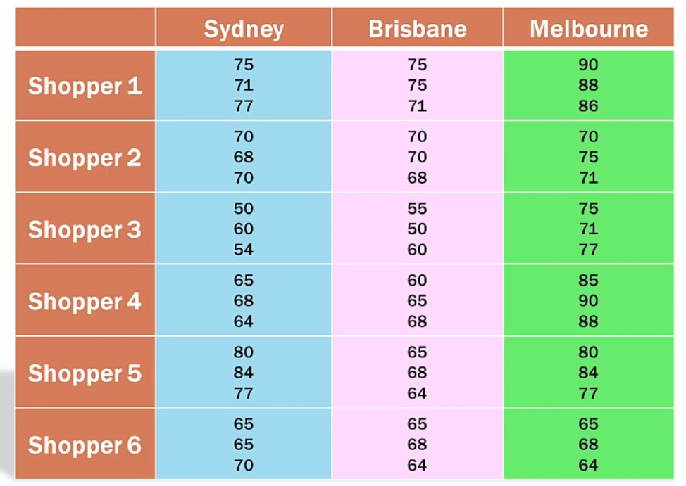
Besides reducing SSE, a two-way ANOVA with replication is mainly used to detect interaction effects between two factors:
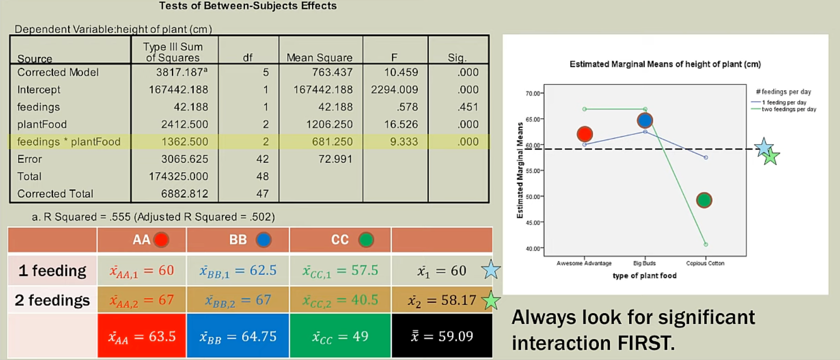
- x-axis = Factor A (main IV); y-axis = DV; line-color = Factor B (group IV)
- We would like to understand whether the effect of one factor (Factor A) on the DV varies across different levels of another factor (Factor B).
- We only focus on the significance of interaction term.
3. ANCOVA
Y ~ X + M + X*M (M is a continuous variable)
One-way ANOVA is used to evaluate whether significant differences exist among the outcomes of various treatments (i.e different levels within a factor). Two-way ANOVA combines two factors within a single study to examine not only the main effects of each factor but also how they interact with each other. To sum up, ANOVA serves as a statistical approach where the predictors are discrete variables (categorical or ordinal). What if we have both discrete and continuous predictors? In such cases, we use ANCOVA.
We can understand the motivation for ANCOVA from two perspectives. First, it can be seen as an improved version of the two-way ANOVA with replication, suitable for a continuous predictor. Thus, its motivation is the same as that of the two-way ANOVA with replication. Second, as indicated by its name, incorporating covariates, or control variables, allows for the exclusion of certain confounding factors.
For more details, please refer to ANCOVA (Analysis of Covariance) in SPSS.
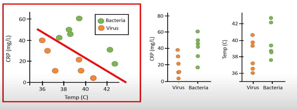
4. MANOVA
ANOVA only has one DV, whereas in MANOVA, there are multiple dependent variables. One possible scenario is that performing MANOVA reveals significant differences between groups, but when conducting separate ANOVAs for each dependent variable, no significant differences are found among the groups:
ANOVA (individual j in group i):
MANOVA:
MANOVA requires checking the homogeneity of the covariance matrices: While ANOVA assumes that the variances of the error terms are the same across all groups, in MANOVA this assumption extends to the covariance matrices. Box’s M test can be used to verify this.