Table of contents
- Motivation
- Model Specification
- Implication: Causal Effects
- Delayed Effects
- Add Control Groups
- References
Motivation
We want to examine whether and how the outcome variable changes after the intervention is implemented. Here, an intervention may be a policy, a program, or another treatment that is implemented at one specific time point. One simple example:
- Y = Number of books read monthly by students in a school
- S = Open a new library
- Question = Does the newly opened library affect the number of books read by students?
There is another advantage of using the interrupted time series (ITS) model: it is relatively simple in many cases. This simplicity means you can draw a fairly valid conclusion with only two things: time and the start date of the intervention.
Model Specification
Three-variable version:
- Time: 1, 2, 3, 4, 5, …
- Treatment: 0, 0, 0, …, 0, 1, 1, 1, 1, 1, …
- Time since treatment: 0, 0, 0, …, 0, 1, 2, 3, 4, 5, …
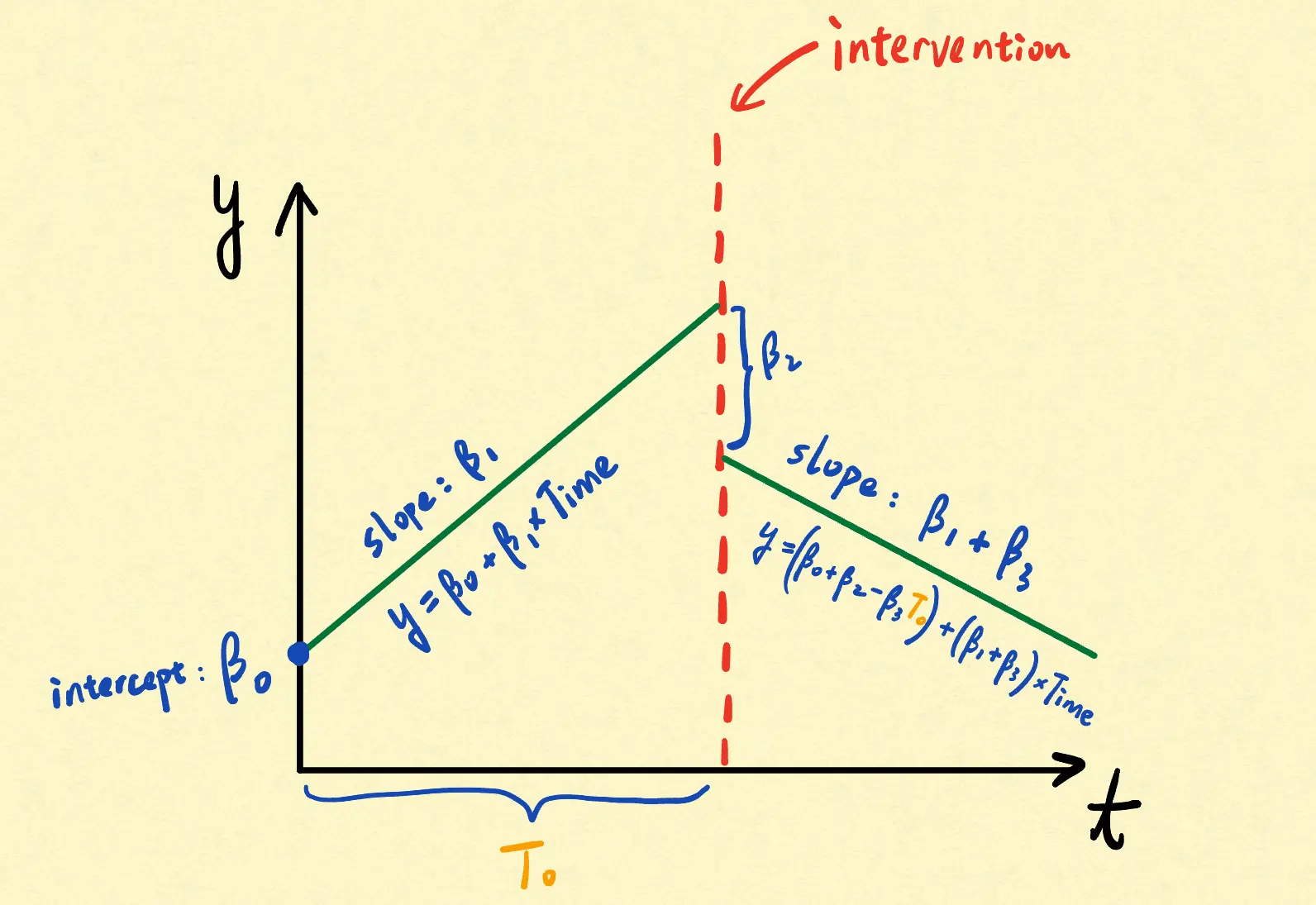
Four possible scenarios for the effect of the intervention:
| Scenarios | Coefficients |
|---|---|
| No effect | β2 = β3 = 0 |
| Only immediate effect (short-term effect) | β2 ≠ 0, β3 = 0 |
| Only sustained effect (long-term effect) | β2 = 0, β3 ≠ 0 |
| Both immediate and sustained effect | β2 ≠ 0, β3 ≠ 0 |
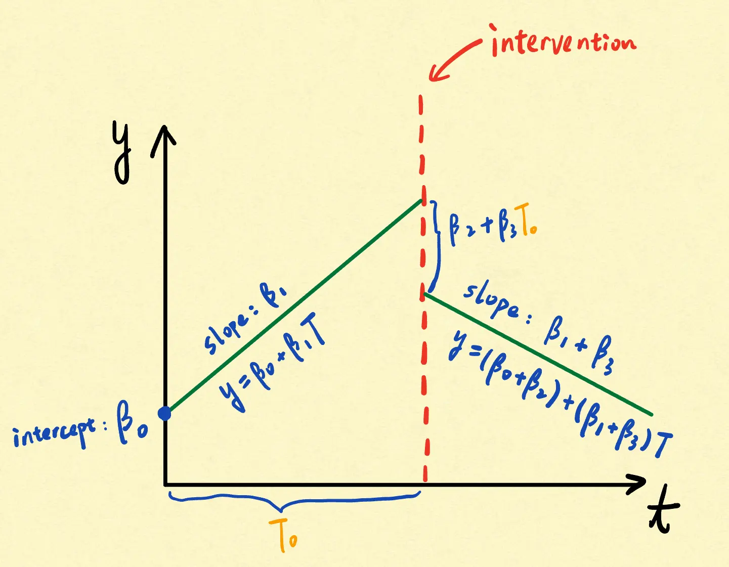
Two-variable version:
- Time: 1, 2, 3, 4, 5, …
- Treatment: 0, 0, 0, …, 0, 1, 1, 1, 1, 1, …
Implication: Causal Effects
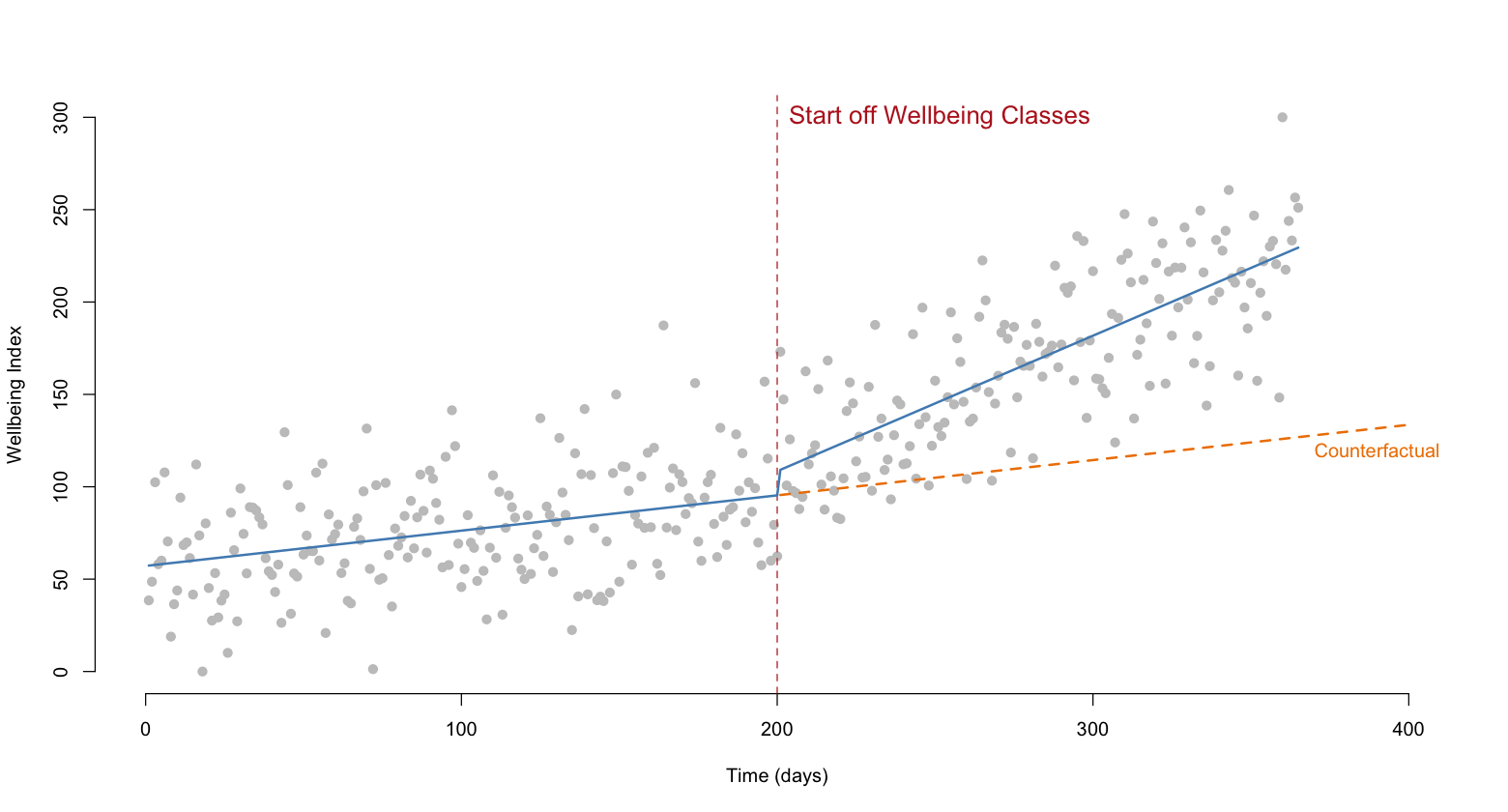
- The ITS model here is used to investigate how the implementation of a mental health program would affect the well-being of students.
- The orange dashed line represents the estimated counterfactual.
- The distance between the blue line after the intervention point and the orange dashed line represents the estimated causal effect.
Delayed Effects
If we suspect a delayed effect, we could examine both immediate and sustained effects several months following the intervention. For example, a fertility policy may not have an immediate effect on the birth rate because a pregnancy lasts at least 9 months.
Add Control Groups
A way to improve internal validity is to add a control group in which individuals are not involved in the intervention. In this case, we could be more confident that the effects observed in the treatment group are caused by the intervention, instead of by other events.