Method | Linear Mixed Models

Gists

Multilevel data: Level 1 model & Level 2 model
Fixed effect ↔ Non-random reg. coef.
Random effect ↔ Random reg. coef. ↔ a restricted version of constructing dummies
It looks like the Bayesian approach that treats parameters as random variables and assigns them prior distributions.

1. Motivation: why does it matter?
2. Model specification & estimation: a theoretical example
3. Fitting a LMM in R: practical examples
- 3.1 Random-intercept model
- 3.2 Introducing random slopes
4. Crossed random effects
References

1. Motivation: why does it matter?

Sometimes, we collect data with multilevel structures. For example, students belong to different schools—students represent Level 1, and schools represent Level 2. When we conduct research on student performance, we can obtain not only the characteristics of the students but also the characteristics of the schools.

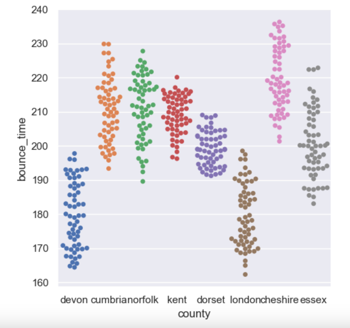
One major issue that multilevel data presents in regression analysis is that observations might not be truly independent. More specifically, observations within each level of Level 2 aren’t independent. As can be seen from the figure below, individuals from the same county are more similar than those from different counties.

There are some approaches to deal with multilevel data other than using a LMM:

Ignoring Level 2 (i.e. Complete pooling): This approach refers to performing a simple linear regression on the entire dataset, which is not ideal. First off, it neglects the dependence among observations, thus violating the assumptions of OLS. Furthermore, it completely overlooks heterogeneity among the levels of Level 2, potentially missing valuable insights from a macro perspective. Such neglect could also lead to poor model fit when examining the data from a within-group perspective.
Aggregation to Level 2: For example, rather than using the individual students’ data, which is not independent, we could take the average of all students within a school. This aggregated data would then be independent. However, the number of data points would decrease dramatically - there would only be 8 data points if it were the situation depicted in the figure.
Separate analysis: This involves fitting a regression model for each level within Level 2. For example, we could run 8 separate linear regressions in the setting of the figure - one for each county. However, the drawbacks are obvious: it completely ignores the inter-group relationships; it also significantly increases the number of parameters to be estimated, wasting degrees of freedom; moreover, the sample size in each separate analysis is drastically reduced, leading to an increase in estimation errors.

LMM can be thought of as a kind of trade off. LMM do not go as far as separate analysis in terms of disaggregation, which means they acknowledge the connections among individuals across groups. On the other hand, LMM allow for a certain degree of variation between different groups regarding the intercept and slopes.

LMM treat some regression coefficients of the Level 1 model as fixed and others as random. This implies that the effect of certain Level 1 explanatory variables is the same across different groups, while the effect of other Level 1 explanatory variables varies between groups - the former are known as fixed effects, and the latter as random effects.

Compared to simple linear regression, where we assume the data are random variables but the parameters are unknown and fixed, some parameters (at Level 1) are modeled as RV in LMM. It is important to note that in the Level 2 (or highest level) model of LMM, all regression coefficients are treated as fixed, which means we still assume some overall population mean. So we can view LMM as an extension of SLR.

2. Model specification & estimation: a theoretical example

Xie, Y., & Hannum, E. (1996). Regional Variation in Earnings Inequality in Reform-Era Urban China. American Journal of Sociology, 101(4), 950–992. https://doi.org/10.1086/230785

This paper examines the factors determining personal income in China, focusing on elements such as education, work experience, Communist Party membership, and gender. Importantly, the article establishes a model of regional heterogeneity: it discusses the impact of urban economic growth on individual income, highlighting the heterogeneity among different cities.

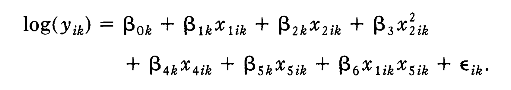
This is the Level 1 model of the LMM: $y_{ik}$ means the income of individual $i$ in city $k$ ； $x_{1ik}$ means years of education of individual $i$ in city $k$ ; $x_{2ik}$ means years of working; $x_{4ik}$ means the membership; $x_{5ik}$ means the gender.

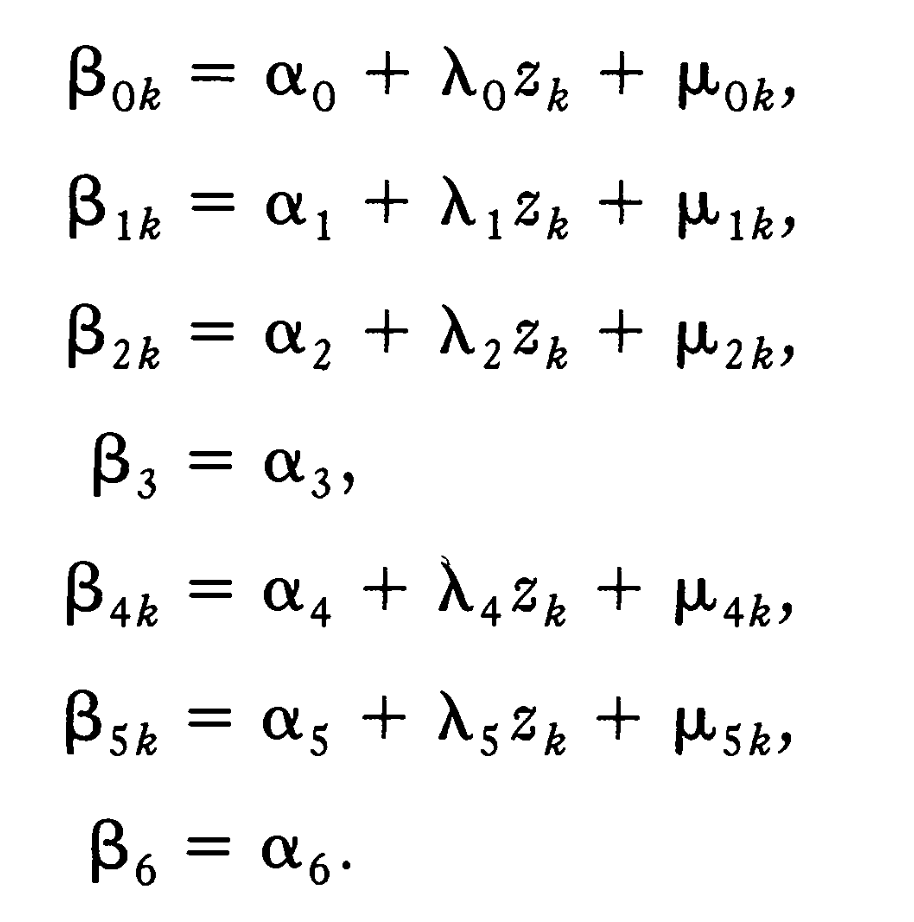
This is the Level 2 model of the LMM: First, we can see that the effect of the square of years of work experience ( $\beta_3$ ) and the interaction effect of years of education and gender ( $\beta_6$ ) are fixed effects, while other effects are random. Second, a Level 2 explanatory variable $z_k$ is used to model all the random effects. $z_k$ refers to the economic change/growth of city $k$ 。In conclusion, this model comprises 2 fixed effects and 5 random effects. Specifically, it treats education, working experience, membership, and gender as random effects, while treating the square term and the interaction term as fixed effects. The model assumptions are:

\epsilon_{ik} \sim_{iid} N(0, \sigma^2) \\ \vec{\mu} \sim_{iid} N(\vec{0}, \Sigma) \\ Cov(\epsilon, \mu) = 0 \text{ for all combinations}

The common estimation method for LMM is MLE (Maximum Likelihood Estimation). In addition to this, there are also IGLS (Iterative Generalized Least Squares) and Bayesian methods. Since there are many available software packages for these methods, they are not described in detail here. Below are the model estimation results from the article:

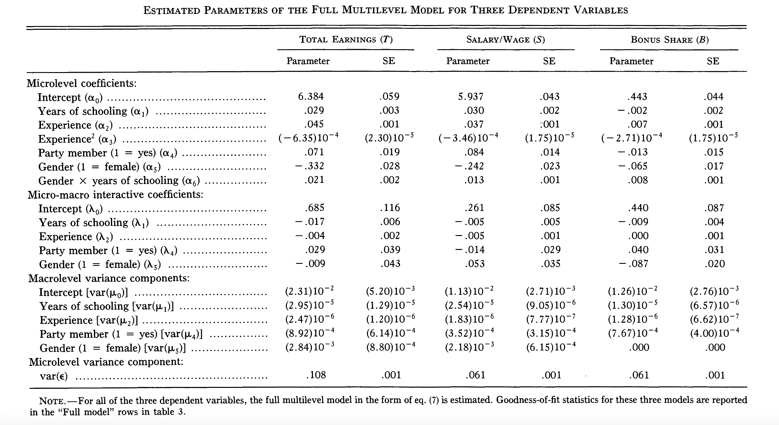
Some interpretations (only focus on the column of TOTAL EARNINGS):

The estimation of $\alpha_0$ is 6.384: for individuals who are male, non-Communist Party members, without education, without work experience, and residing in cities with no economic growth, the average income is exp(6.384) = 592.3 yuan.
The estimation of $\lambda_0$ is 0.685: the model posits that the Level 1 intercept can vary by city, a variation represented by a significantly non-zero λ0. This suggests that in cities with higher economic growth, the baseline income tends to be higher.
The estimation of $\alpha_1$ is 0.029: controlling for the city’s economic growth, the effect of years of education on total income is 0.029 for men. For women, combining the estimated value of α6, the effect of years of education on total income is 0.029 + 0.021 = 0.050.
The estimation of $\lambda_1$ is -0.017: the effect of education on total income is negatively correlated with the economic growth of a city. However, considering the range of values for z in the sample, this correlation does not reverse the sign of the effect of education on total income.
$\lambda_4$ is not significant: there is no significant relationship between the effect of Communist Party membership on total income and the economic growth of a city.
$\lambda_5$ is not significant: there is no significant relationship between the effect of gender on total income and the economic growth of a city.

Additionally, the article quantitatively explains why it is important to consider a regional heterogeneity model. First, it establishes a random coefficient model—where no explanatory variables are introduced in the Level 2 model, meaning that all random effects have only a random component without any systematic component. The fitting results are shown in the figure below:

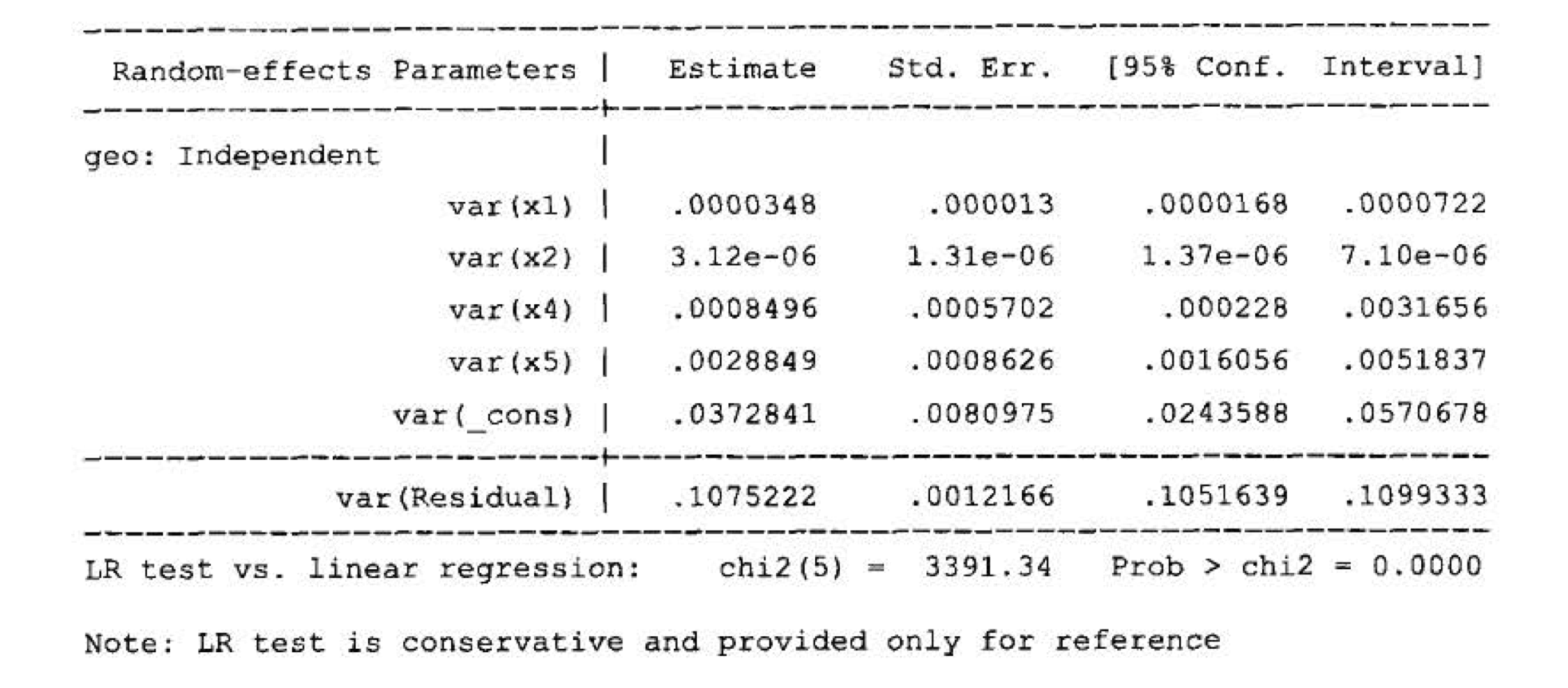
It is evident that the variance of all random effects is significantly non-zero, as the confidence intervals do not include zero. This suggests that the assumption of the existence of random effects is reasonable. Therefore, it may be necessary to identify some city-level factors to further explain these random effects, rather than solely using a random component. Consequently, the explanatory variable $z$ at Level 2 is introduced.

3. Fitting a LMM in R: practical examples

library(lme4)

3.1 Random-intercept model

A random-intercept model implies that only the intercept in the Level 1 model is random, while other slopes are fixed. Take this tutorial as an example:

Q: how does the body length of the dragons affect their test scores?
Individuals are sampled with a range of body lengths in 8 different mountain ranges.
Level 1: IV=body length, DV=test score; Level 2: mountain range
The effect of body length is treated as a fixed effect; the intercept is viewed as random without systematic components.

y_{ik} = \beta_{0k} + \beta_{1k} x_{ik} + \epsilon_{ik}\\ \beta_{0k} = \alpha_0 + \mu_{0k}\\ \beta_{1k} = \alpha_1

This implies a consistent relationship between body length and intelligence across dragons in various mountain ranges (fixed slope), but also recognizes the potential for inherent intelligence differences among different dragon populations (random intercept). The combined model:

y_{ik} = \alpha_0 + \alpha_1 x_{ik} + \mu_{0k} + \epsilon_{ik}

So we have (just like variance decomposition in ANOVA):

Var(y_{ik}) = Var(\mu_{0k}) + Var(\epsilon_{ik})

# (1|mountainRange) can be interpreted as
# “intercept varies across different mountainRange”
mixed.lmer = lmer(testScore ~ bodyLength2 + (1|mountainRange), data = dragons)
summary(mixed.lmer)

3.2 Introducing random slopes

Take this tutorial as an example:

Q: does reaction time increase or decrease with increasing sleep deprivation?
Each individual underwent measurements for ten consecutive days.
Level 1: IV=days_deprived, DV=reaction_time; Level 2: subject
The effect of days_deprived is treated as a random effect; the intercept is viewed as random without systematic components.

y_{sd} = \beta_{0s} + \beta_{1s} x_{sd} + \epsilon_{sd}\\ \beta_{0s} = \alpha_0 + \mu_{0s}\\ \beta_{1s} = \alpha_1 + \mu_{1s}\\

In this context, the random slope means that the impacts of sleep deprivation vary among individuals; while some may be highly susceptible to its effects, others may demonstrate resilience; this variability is not attributable to systematic factors like individual characteristics. The combined model:

y_{sd} = \alpha_0 + \alpha_1x_{sd}+ \mu_{0s} + x_{sd}\mu_{1s} + \epsilon_{sd}

# (days_deprived | Subject) can be interpreted as
# “intercept and the effect of days_deprived
# varies across different Subject
# another equivalent syntax: (1 + days_deprived | Subject)
pp_mod = lmer(Reaction ~ days_deprived + (days_deprived | Subject), data = sleep2)
summary(pp_mod)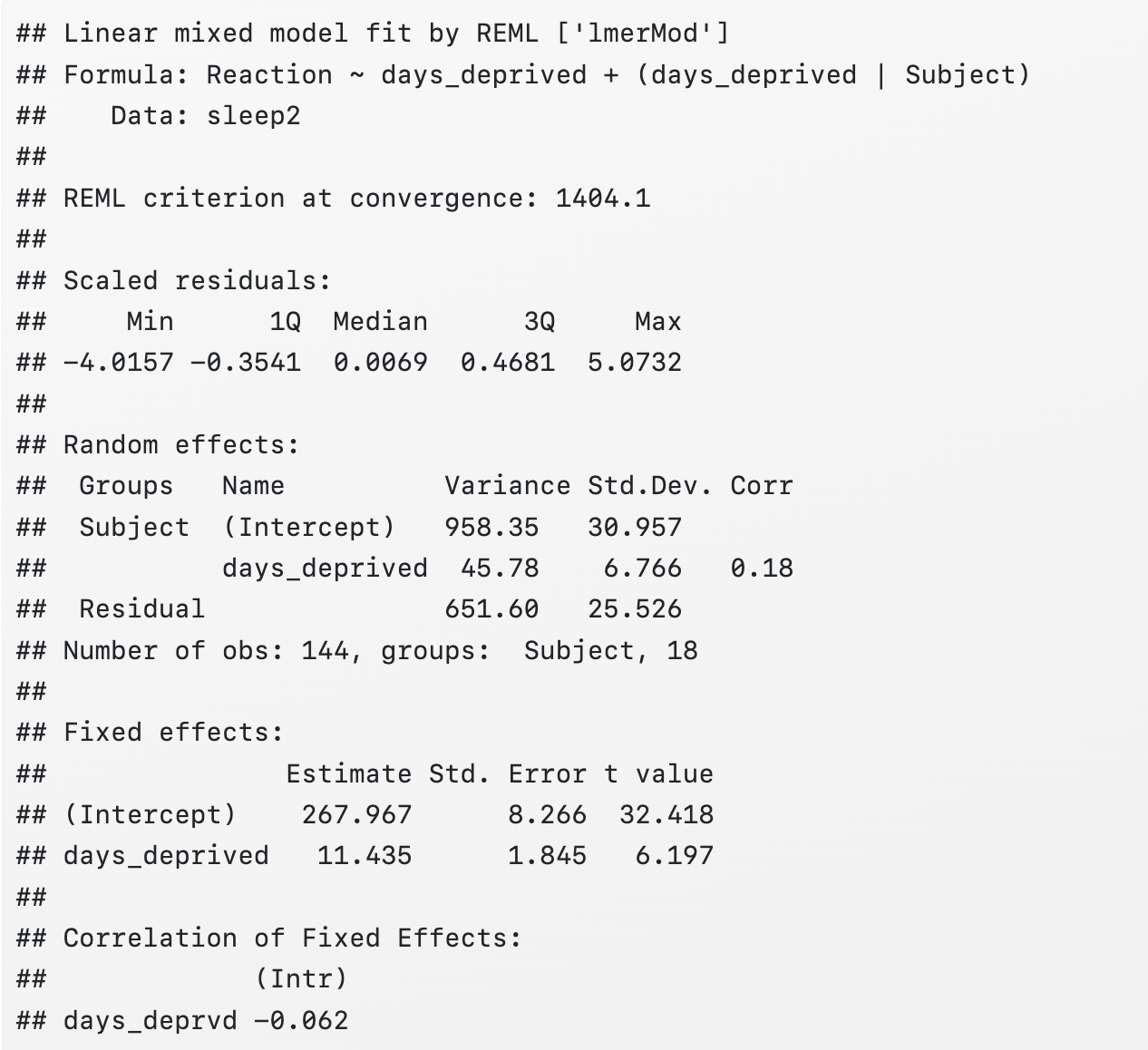

“Fixed effects” part: “This indicates that the estimated mean reaction time for participants at Day 0 was about 268 milliseconds, with each day of sleep deprivation adding an additional 11 milliseconds to the response time, on average.”
“Random effects” part:
- (Intercept) = 958.35 → estimation of $Var(\mu_{0s})$
- days*deprived = 45.78 → estimation of $Var(\mu*{1s})$
- Corr = 0.18 → estimation of $Corr(\mu_{0s}, \mu_{1s})$

4. Crossed random effects

Many experiments in psychology often aim to answer this type of question: “what happens to our measurements when an individual of type X encounters a stimulus of type Y”, where X is drawn from a target population of subjects and Y is drawn from a target population of stimuli (i.e. items).

In this context, there appear to be two distinct Level 2 groupings. First, data points can be grouped based on subjects, and secondly, they can be grouped according to items. This differs from the nested Level scenario, such as a leaf within a tree within a field, where the grouping levels are clearly nested within each other.

For example, there is an experiment involving lexical decisions to a set of words (e.g., is “PINT” a word or nonword?), and the dependent variable is response time, and the independent variable is word type (noun vs verb). The model / data generating process:

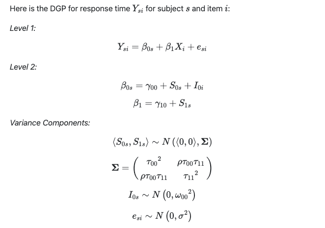
random intercept: variations from both items and subjects - they are independent
random slope: only variation from subjects

In R, you should specify your model as following:

mod = lmer(Y ~ cond + (1+cond | subj_id) + (1 | item_id), data)