Method | Mediation Analysis (in R)

1. Model specification
2. Baron & Kenny’s 4-step method
- 2.1 Four steps
- 2.2 Example
3. Test significance of indirect effect
4. Paper Reproduction
Reference

1. Model specification

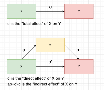
M is a mediator showing the ’how’ or ’why’ of the relationship between X and Y - a mediator reveals the causal mechanism linking X and Y.
A mediation model is a causal model grounded in theoretical construction. We typically first hypothesize the model and then test its statistical significance, rather than defining the model statistically. In other words, if the assumed causal model is incorrect, the results obtained from the mediation analysis are likely to be of limited value.
Direct effect is simply the direct relationship between X and Y in presence of M ( $c'$ $c^{'}$ ); Indirect effect is the relationship that flows from X to M and then to Y ( $a \times b$ $a \times b$ ); Total effect is the combined influence of the direct effect and the indirect effect ( $c \equiv c'+a \times b$ $c \equiv c^{'} + a \times b$ ).
- There is another way to measure the indirect effect, $(a \times b)/c$ , which represents the proportion of the total effect that is mediated by M. However, the product of coefficients ( $a \times b$ ) is more commonly used.

2. Baron & Kenny’s 4-step method

2.1 Four steps

This is the original and simple method to evaluate a mediation effect:

Step 1: X ~ Y
- X must be correlated with Y. Otherwise, there is no effect to mediate.
- However, this can be violated with a “suppressive mediator(抑制)“.
- Hence, step 1 is not that important.
Step 2: X ~ M
- X must be correlated with M (path a).
Step 3: Y ~ X + M
- M must be correlated with Y when controlling X (path b).
Step 4: evaluate the direct effect in step 3 (path c’)
- X no longer correlates with Y → Complete mediation
- X correlates with Y, but the magnitude is reduced → Partial mediation

2.2 Example

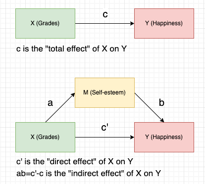
This toy example is derived from Introduction to Mediation Analysis:

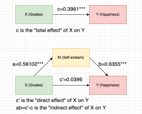
# Step 1: Total effect = Path c = 0.3961***
model.0 = lm(Y ~ X, data=myData)
summary(model.0)

Call:
lm(formula = Y ~ X, data = myData)

Residuals:
    Min      1Q  Median      3Q     Max
-5.0262 -1.2340 -0.3282  1.5583  5.1622

Coefficients:
            Estimate Std. Error t value Pr(>|t|)
(Intercept)   2.8572     0.6932   4.122 7.88e-05 ***
X             0.3961     0.1112   3.564 0.000567 ***
---
Signif. codes:  0 ‘***’ 0.001 ‘**’ 0.01 ‘*’ 0.05 ‘.’ 0.1 ‘ ’ 1

Residual standard error: 1.929 on 98 degrees of freedom
Multiple R-squared:  0.1147,	Adjusted R-squared:  0.1057
F-statistic:  12.7 on 1 and 98 DF,  p-value: 0.0005671

# Step 2: Path a = 0.56102***
model.XM = lm(M ~ X, data=myData)
summary(model.XM)

Call:
lm(formula = M ~ X, data = myData)

Residuals:
    Min      1Q  Median      3Q     Max
-4.3046 -0.8656  0.1344  1.1344  4.6954

Coefficients:
            Estimate Std. Error t value Pr(>|t|)
(Intercept)  1.49952    0.58920   2.545   0.0125 *
X            0.56102    0.09448   5.938 4.39e-08 ***
---
Signif. codes:  0 ‘***’ 0.001 ‘**’ 0.01 ‘*’ 0.05 ‘.’ 0.1 ‘ ’ 1

Residual standard error: 1.639 on 98 degrees of freedom
Multiple R-squared:  0.2646,	Adjusted R-squared:  0.2571
F-statistic: 35.26 on 1 and 98 DF,  p-value: 4.391e-08

# Step 3 & 4: Path b + Path c'
#             Path b = 0.6355***
#             Path c'= 0.0396
model.MY.XY = lm(Y ~ X + M, data=myData)
summary(model.MY.XY)

Call:
lm(formula = Y ~ X + M, data = myData)

Residuals:
    Min      1Q  Median      3Q     Max
-3.7631 -1.2393  0.0308  1.0832  4.0055

Coefficients:
            Estimate Std. Error t value Pr(>|t|)
(Intercept)   1.9043     0.6055   3.145   0.0022 **
X             0.0396     0.1096   0.361   0.7187
M             0.6355     0.1005   6.321 7.92e-09 ***
---
Signif. codes:  0 ‘***’ 0.001 ‘**’ 0.01 ‘*’ 0.05 ‘.’ 0.1 ‘ ’ 1

Residual standard error: 1.631 on 97 degrees of freedom
Multiple R-squared:  0.373,	Adjusted R-squared:  0.3601
F-statistic: 28.85 on 2 and 97 DF,  p-value: 1.471e-10

Results:

Interpretation:

The total effect model shows a significant positive relationship between grades(X) and happiness(Y).
- Path c = 0.3961***
The path a model shows grades(X) positively correlate with self-esteem(M) and the relationship is statistically significant.
- Path a = 0.56102***
Self-esteem(M) positively predicts happiness(Y) when controlling grades(X). At the same time, the relationship between grades(X) and happiness(Y) is no longer significant.
- Path b = 0.6355***
- Path c’= 0.0396
This suggests that self-esteem(M) completely mediates the relationship between grades(X) and happiness(Y).
- However, this method cannot directly evaluate the significance of the indirect effect (i.e. ab≠0) - we need a formal test for a statistical verification.

3. Test significance of indirect effect

This is the null hypothesis that we want to test:

H_0: ab=0

>>> Code for this section

3.1 Naive method: joint significance of paths a and b

Test whether both path a and path b are significantly different from 0. If so, the indirect effect is probably non-zero and we could reject the null hypothesis.

👍 work rather well, but rarely used as the definitive test; Use this test in conjunction with other tests.
👎 major drawback: does not provide a confidence interval for the indirect effect.

Based on this criterion, we could conclude that the indirect effect between grades(X) and happiness(Y), $ab=0.5610×0.6355=0.3565$ , is significantly different from 0 because both path a and path b are significant.

3.2 Delta method: Sobel test

The Delta method represents a group of tests that construct a standard normal distributed statistic based on the standard error of $\hat{a}\hat{b}$ . And Sobel test is by far the most commonly used one. The test statistic:

\frac{\hat{a} \cdot \hat{b}}{\sqrt{\hat{a}^2 \cdot se(\hat{b})^2 + \hat{b}^2 \cdot se(\hat{a})^2}}

All the values in the formula can be accessed through step 2 and 3.
The denominator is the standard error of $\hat{a}\hat{b}$ .
When H0 is true, the test statistic follows standard normal distribution.
👍 easy to compute.
👎 very conservative (i.e. low power; not easy to reject H0) because the sampling distribution of ab is higly skewed (but Sobel test assumes the sampling distribution is normal distribution).

Based on Sobel test, we could compute the p-value (p=1.505e-05) and reject the H0 accordingly, which refers to a significant indirect effect. We can also compute a 95% confidence interval for the indirect effect ab ( $0.3565 \plusmn 1.96 \times 0.0824$ ), which does not include 0:

[0.1950, 0.5180]

Code in R:

######## 手动计算: https://www.spss-tutorials.com/sobel-test-what-is-it/
alpha = summary(model.XM)$coefficients["X","Estimate"]
se_alpha = summary(model.XM)$coefficients["X","Std. Error"]
beta = summary(model.MY.XY)$coefficients["M","Estimate"]
se_beta = summary(model.MY.XY)$coefficients["M","Std. Error"]

z.statistic = (alpha * beta)/(sqrt(alpha*alpha*se_beta*se_beta + beta*beta*se_alpha*se_alpha))
p.value = 2*(1-pnorm(z.statistic))  # two-tailed

sprintf("indirect effect: %s", alpha*beta)
sprintf("z-statistic: %s", z.statistic)
sprintf("p-value: %s", p.value)

######## 使用函数
library(multilevel)
sobel(myData$X, myData$M, myData$Y)

3.3 Resampling method: bootstrapping

The resampling method represents a group of approaches based on sampling techniques. For example, bootstrapping, which means resampling with replacement many times, could empirically generate a sampling distribution. Then, we can compute an approximate standard deviation of $\hat{a}\hat{b}$ and construct a confidence interval. If 0 is not in the interval, we can conclude that the indirect effect is significant. We can use mediation or lavaan package to implement resampling methods in R.

3.3.1 `mediation`

Doc (Tingley, Yamamoto, Hirose, Keele, & Imai, 2014)
The default simulation type is the quasi-Bayesian Monte Carlo method.
By setting boot = TRUE, we can use the bootstrapping (sims >= 1000).

res.1 = mediate(model.XM, model.MY.XY, treat='X', mediator='M',
                boot=TRUE, sims=1000)
summary(res.1)

Causal Mediation Analysis

Nonparametric Bootstrap Confidence Intervals with the Percentile Method

              Estimate 95% CI Lower 95% CI Upper p-value
ACME             0.3565       0.2199         0.53  <2e-16 ***
ADE              0.0396      -0.2218         0.29    0.82
Total Effect     0.3961       0.1558         0.65  <2e-16 ***
Prop. Mediated   0.9000       0.4849         2.32  <2e-16 ***
---
Signif. codes:  0 ‘***’ 0.001 ‘**’ 0.01 ‘*’ 0.05 ‘.’ 0.1 ‘ ’ 1

Sample Size Used: 100


Simulations: 1000

Interpreting results:

ACME即Average Causal Mediation Effects，也即indirect effect。
ADE即Average Direct Effects，也即direct effect。
Total Effect就是total effect。

3.3.2 `lavaan`

# Step 1: Specify mediation model
# The lavaan syntax
model = "
# Path c' (direct effect)
Y ~ c*X
# Path a
M ~ a*X
# Path b
Y ~ b*M
# Indirect effect (a*b)
ab := a*b
"

# Step 2: Estimate model - delta method (by default)
fitmod = sem(model, data=myData)
# Step 3: Request summary
summary(fitmod, fit.measures=TRUE, rsquare=TRUE)

Regressions:
                  Estimate  Std.Err  z-value  P(>|z|)
  Y ~ X        (c)    0.040    0.108    0.367    0.714
  M ~ X        (a)    0.561    0.094    5.998    0.000
  Y ~ M        (b)    0.635    0.099    6.418    0.000

Variances:
                  Estimate  Std.Err  z-value  P(>|z|)
  .Y                 2.581    0.365    7.071    0.000
  .M                 2.633    0.372    7.071    0.000

R-Square:
                  Estimate
    Y                 0.373
    M                 0.265

Defined Parameters:
                  Estimate  Std.Err  z-value  P(>|z|)
    ab                0.357    0.081    4.382    0.000

Interpreting lavaan results:

“Y ~ X (c)” is the direct effect - not significant
“M ~ X (a)” is the path a - significant
“Y ~ M (b)” is the path b - significant
“defined para: ab” is the indirect effect - significant
R-Square:
- X and M explain 37.3% variation of Y.
- X explains 26.5% variation of M.

# Step 2: Estimate model - percentile bootstrapping method
fitmod2 = sem(model, data=myData, se="bootstrap", bootstrap=1000)
# Ste[pRequest percentile bootstrap 95% confidence intervals
parameterEstimates(fitmod2, ci=TRUE, level=0.95, boot.ci.type="perc")

  lhs op rhs label   est    se     z pvalue ci.lower ci.upper
1   Y  ~   X     c 0.040 0.125 0.316  0.752   -0.217    0.280
2   M  ~   X     a 0.561 0.096 5.848  0.000    0.375    0.773
3   Y  ~   M     b 0.635 0.102 6.223  0.000    0.428    0.831
4   Y ~~   Y       2.581 0.324 7.977  0.000    1.886    3.168
5   M ~~   M       2.633 0.354 7.434  0.000    1.928    3.312
6   X ~~   X       3.010 0.000    NA     NA    3.010    3.010
7  ab := a*b    ab 0.357 0.080 4.467  0.000    0.206    0.540

Method | Mediation Analysis (in R)

Table of contents