Statistics | Proportional-odds Logistic Regression

1. Motivation
2. Model Specification
3. Checking Model Fit
4. Interpretation of Coefficients
- 4.1. General Interpretation
- 4.2. An Example
5. References

1. Motivation

TBD. Here, we are using the proportional-odds model, which models cumulative probabilities. This model has many names:

Proportional-odds model
Proportional odds logistic regression
Proportional-odds cumulative logit model
Cumulative logit model
Ordinal/Ordered logistic regression with proportional odds assumption

2. Model Specification

2.1. Cumulative Logits

Suppose the outcome variable Y is an ordinal with ordered categories 1 to J:

Y \in \{1,2,\cdots,J\}

Model the logit (i.e. log odds) of the cumulative probabilities for J-1 categories:

\text{logit} [P(Y\le j|\mathbf{x})] = \log \bigg(\frac{P(Y\le j|\mathbf{x})}{1-P(Y \le j|\mathbf{x})}\bigg) := \alpha_j + \beta^T\mathbf{x}\\ j = 1,2,\cdots,J-1

Only J-1 categories because $P(Y \le J |\mathbf{x} )=1$
Separate intercept but shared slope for each cumulative logit
#Params: (J-1) intercepts + 1 slope

2.2. Proportional Odds Assumption

For “each way to collapse Y into a binary outcome” (i.e., for each category), the log odds ratio equals to $\beta^T\Delta \mathbf{x}$ >>> i.e., the log odds ratio is proportional to the difference between x1 and x2 - And the proportionality coefficient is constant:

\text{logit} [P(Y\le j|\mathbf{x}_1)]-\text{logit} [P(Y\le j|\mathbf{x}_2)]=\beta^T(\mathbf{x}_1-\mathbf{x}_2)\\ \text{LHS}=\log(\frac{odds(Y\le j|\mathbf{x}_1)}{odds(Y\le j|\mathbf{x}_2)})

“The effect of x is the same for all C-1 ways to collapse Y into dichotomous outcomes.”
“A single parameter describes the effect of x on Y.” (however, in the multinominal logit model, there is C-1 βs).

2.3. Model Graph

Suppose there is only one predictor X, and J=4:

\pi_j(x) = P(Y=j|x)

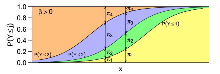
Each curve represents $P(Y \le j |x)$ .
Curves are parallel >>> do not cross over.

3. Checking Model Fit

3.1. Compare to the “Unparalleled” Model

i.e., Test of Proportional Odds Assumption

H_0: \text{The proportional odds assumption holds}

## Fit ordered logit model with parallel assumption
model.1 <- vglm(ses ~ science + socst + female,
                family = cumulative(parallel = TRUE, link = "logitlink"),
                data = df)

## Fit ordered logit model without parallel assumption
model.2 <- vglm(ses ~ science + socst + female,
                family = cumulative(parallel = FALSE, link = "logitlink"),
                data = df)

chi.stat <- 2*(logLik(model.2) - logLik(model.1))
df.delta <- df.residual(model.1) - df.residual(model.2)
print(chi.stat)
print(df.delta)
print(1 - pchisq(chi.stat, df.delta))

The unparalleled model = model without parallel assumption = $\beta_j$ instead of $\beta$
Likelihood ratio test
We want to have p-value > 0.05

3.2. Compare to the Saturated Model

i.e., Test of Goodness-of-fit

H_0: \text{The model fits data well}

## Fit ordered logit model with parallel assumption
model.1 <- vglm(ses ~ science + socst + female,
                family = cumulative(parallel = TRUE, link = "logitlink"),
                data = df)

## Get deviance
devi <- deviance(model.1)
print(devi)

## Get df for null distribution (#params of saturated - #params of this model)
df.delta <- df.residual(model.1)
print(df.delta)

## Get p-value
print(1 - pchisq(devi, df.delta))

We want to have p-value > 0.05
However, this test is only reliable when it is grouped data, or even grouped data with most of the fitted counts are greater than 5.

3.3. Compare to the Null Model

H_0: \text{The null model is good (all β = 0)} \\ H_1: \text{This model is good (at least one β != 0)}

## Fit ordered logit model with parallel assumption
model.1 <- vglm(ses ~ science + socst + female,
                family = cumulative(parallel = TRUE, link = "logitlink"),
                data = df)

## Overall test
lrtest(model.1)

The null model = intercept-only model
Likelihood ratio test
We want to have p-value < 0.05

4. Interpretation of Coefficients

4.1. General Interpretation

Reformulate the model:

P(Y\le j|x) = \frac{1}{1+\exp (-(\alpha_j + \beta x))}

$\beta >0$ → x increases, P(Y≤j) increases regarding a fixed j → x increases, Y is more likely to be in a lower category.
$\beta <0$ → x increases, P(Y≤j) decreases regarding a fixed j → x increases, Y is more likely to be in a higer category.
For every 1-unit increase in x, the odds ratio of Y≤j is exp(β) for each category j.
- or, the odds of Y≤j become exp(β) times as large as the original.
- Odds越大，也就是Prob越大。
Given a specific x, we can compute the estimated probability of y falling into J categories respectively.

4.2. An Example

Variable	Type	Values	Description
ses (DV)	Ordinal	low-1, medium-2 and high-3	socio-economic status
science (IV)	Ratio	>0	science test scores
socst (IV)	Ratio	>0	social science test scores
female (IV)	Nominal	male-0, female-1	gender

df        <- read_sas("./data/hsb2.sas7bdat")
df$female <- factor(df$female, levels = c(0, 1))
df$ses    <- factor(df$ses, levels = c(3, 2, 1), ordered = TRUE)

model <- vglm(ses ~ science + socst + female,
              family = cumulative(parallel = TRUE, link = "logitlink"),
              data = df)

Why not use levels = c(1, 2, 3) here? Because if we do, a positive β (β > 0) would imply that as x increases, an individual is more likely to be in a lower socio-economic (S-E) status. However, we want the interpretation to be the opposite—where a positive β indicates a higher likelihood of being in a higher S-E status. To achieve this, we reverse the order when constructing the factor.

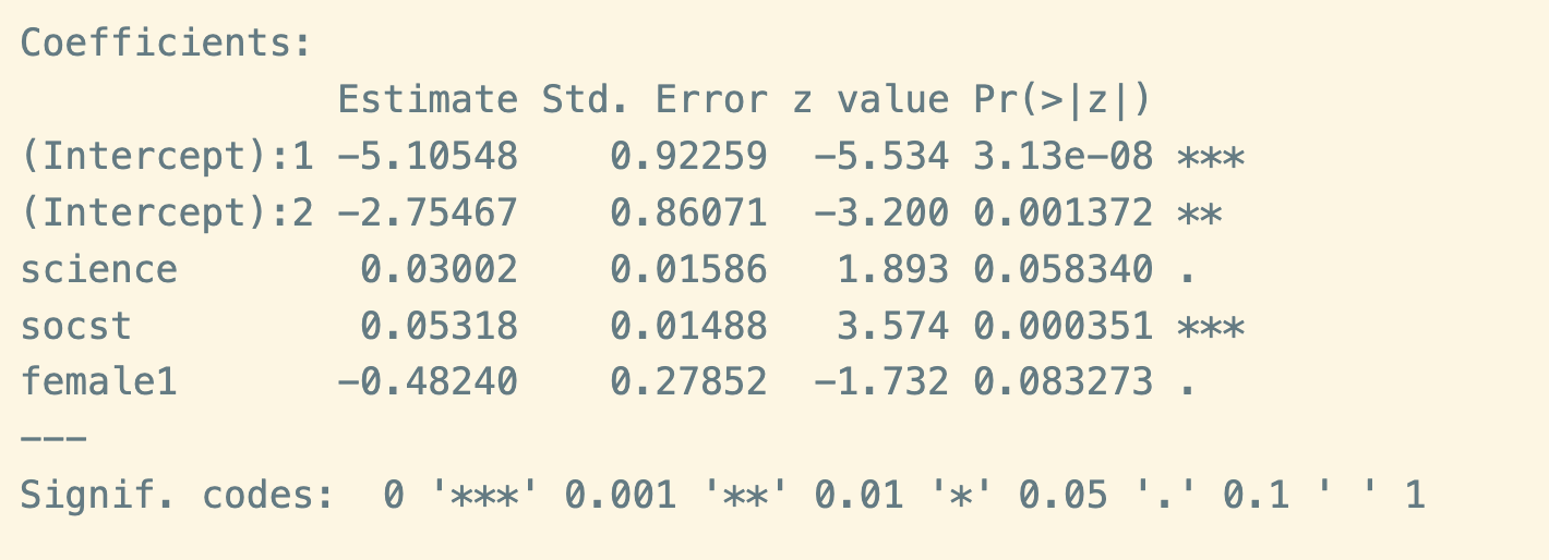
Intercept 1 (-5.11***)
- Estimated log odds for (high ses) versus (low and middle ses) when the predictors are evaluated at zero.
- The log odds of (high ses) versus (low and middle ses) for a male with a zero science and socst test score is -5.11.
Intercept 2 (-2.75**)
- Estimated log odds for (high and middle ses) versus (low ses) when the predictors are evaluated at zero.
- The log odds of (high and middle ses) versus (low ses) for a male with a zero science and socst test score is -2.75.
science (0.03)
- 【直接解释】1) For a one unit increase in science test score, the odds of (high ses) are exp(0.03)=1.03 times greater than for the combined effect of (middle and low ses) given the all the other variables are held constant. 2) Likewise, for a one unit increase in science test score, the odds of (middle and high ses) versus (low ses) is exp(0.03)=1.03 times greater given all the other variables are held constant.
- 【简便解释】在其他predictors不变的前提下，science test score每增加1分，log odds of (higher ses) versus (lower ses)增加0.03 >>> odds of being in higher ses变为原来的exp(0.03)=1.03倍 >>> science test score增加，高阶层概率增加。
socst (0.05***)
- 在其他predictors不变的前提下，social science test score每增加1分，log odds of (higher ses) versus (lower ses)增加0.05 >>> odds of being in higher ses变为原来的exp(0.05)=1.05倍 >>> social science test score增加，高阶层概率增加。
female (-0.48)
- 在其他predictors不变的前提下，女性(female=1)相较于男性(female=0)，log odds of (higher ses) versus (lower ses)降低0.48 >>> odds of being in higher ses变为原来的exp(-.48)=0.62倍 >>> 女性相对于男性，高阶层概率降低。

5. References

[UCLA] Ordinal logistic regression in R with an example: https://stats.oarc.ucla.edu/r/dae/ordinal-logistic-regression/
[UCLA] Ordinal logistic regression in SAS with a detailed example: https://stats.oarc.ucla.edu/sas/output/ordered-logistic-regression/
[PSU] The Proportional-Odds Cumulative Logit Model (& Adjacent-Category Logits): https://online.stat.psu.edu/stat504/lesson/8/8.4
[UI] Cumulative logit model & Adjacent categories logit model: https://education.illinois.edu/docs/default-source/carolyn-anderson/edpsy589/lectures/8_Multicategory_logit/ordinal_logistic_post.pdf
[Uchicago] Cumulative Logit Models for Ordinal Responses: https://www.stat.uchicago.edu/~yibi/teaching/stat226/2023/L21.pdf
[Paper] Regression Models with Ordinal Variables: https://scholar.harvard.edu/files/cwinship/files/asr_1984.pdf