Statistics | Regression Diagnostics

1. For Linear Regression
2. For Logistic Regression
3. References

1. For Linear Regression

1.1. Assumptions for LR

Linearity: The mean of the dependent variable (DV), given the predictors, is a linear function of the predictors.
Independence, Normality, and Equal Variance: The error terms are independently and identically distributed (i.i.d.) from $N(0,\sigma^2)$ $N (0, σ^{2})$ .
- To be more precise, the normality and equal variance assumptions are “conditional version” - at each X, the error terms are normally distributed and have same variances.
No Extreme Points: should be regarded as an additional assumption.

1.2. Residuals-Fitted Values Plot

A “healthy” plot should look like the following ones:

1) Residuals should randomly bounce above and below 0 (i.e. symmetry) >>> Linearity. The following plot indicates a violation, suggesting that the relationship between Y and Xs might not be linear:

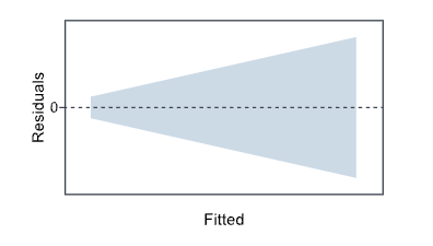
2) Residuals are distributed within a horizontal band centered around 0 >>> Equal variances. The following plot indicates a violation, suggesting that variances of error might not be constant.

3) No residuals deviate drastically from the basic pattern >>> No outliers.

Remark: You can also plot a series of scatterplots with residuals on the y-axis and each predictor on the x-axis (i.e. Residuals-Predictors Plot). These plots function similarly to the Residuals-Fitted Values Plot, and the judging criteria are the same. A violation in at least one plot suggests that you should apply some transformations.

In R, we can use plot(model.1, which = 1) to generate the Residuals-Fitted Values Plot.

1.3. Plot Residuals Only

Plot a histogram, boxplot, or normal probability plot of the residuals to check for Normality.

Normal probability plot: If the data follow a normal distribution, then a plot of the theoretical percentiles of the normal distribution versus the observed sample percentiles should be approximately linear. In this case, this plot is also called “Q-Q plot.”

Some indications for violations:

1) Skewed residuals

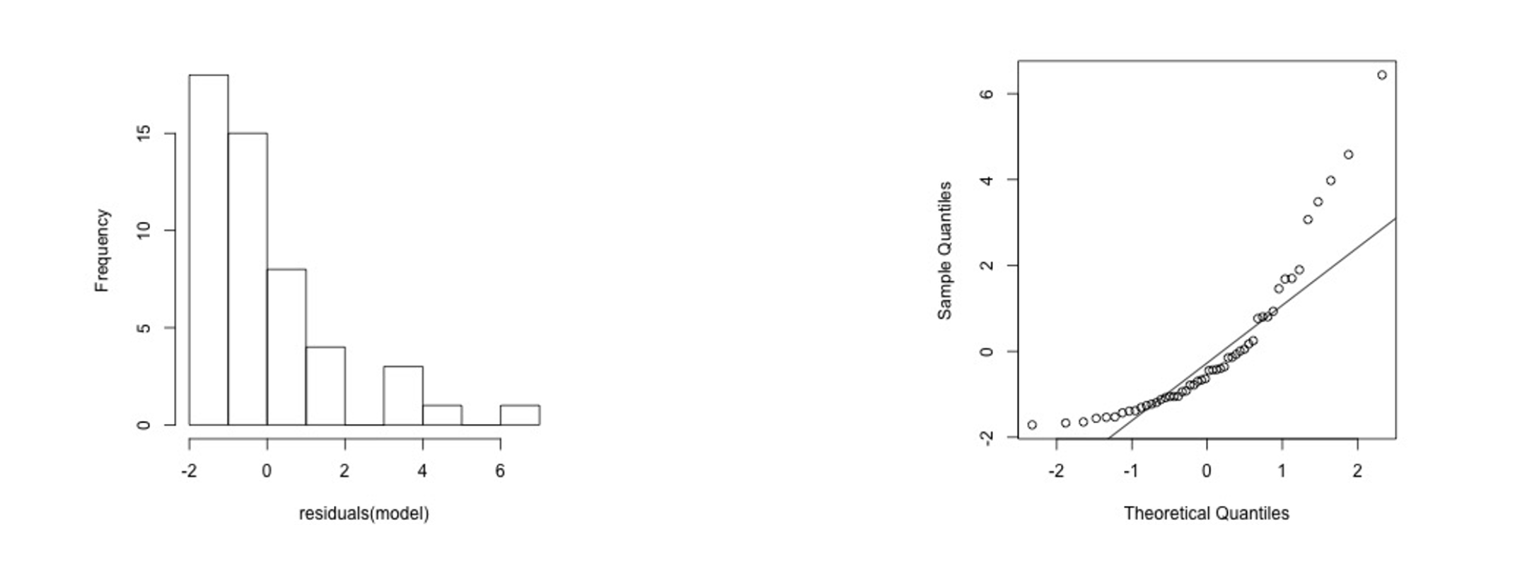
On the Q-Q plot, it mainly appears as larger sample quantiles on both ends.

2) Heavy-tailed residuals

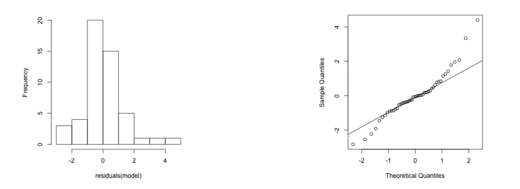
On the Q-Q plot, it mainly appears as a smaller sample quantile on the far left and a larger sample quantile on the far right.

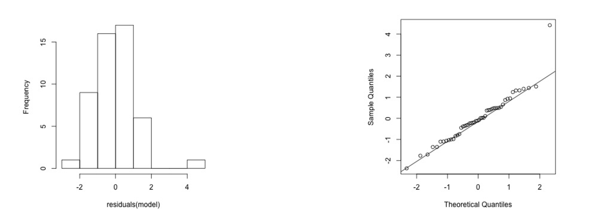
3) Normal residuals but with one outlier

In R,

## Generate Q-Q Plot
plot(model, which = 2)

# Histogram of residuals
hist(residuals(model),
     main = "Histogram of Residuals", xlab = "Residuals")

# Boxplot of residuals
boxplot(residuals(model),
        main = "Boxplot of Residuals", ylab = "Residuals", horizontal = TRUE)

1.4. Identify Influential Points

Influential data points can affect any part of the regression analysis, leading to significantly different results depending on their inclusion. Two sources of being influential: 1) high-leverage points (i.e., have extreme X values), 2) outliers (i.e., have Y values that do not follow the general trent of the rest of the data):

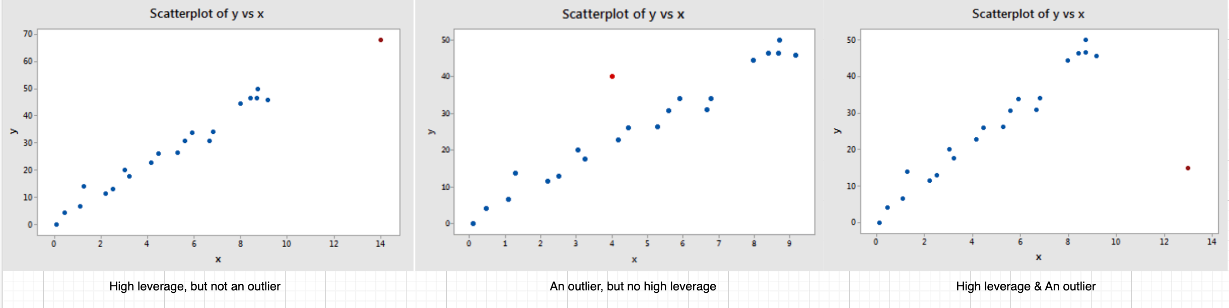
High-leverage points and outliers are not necessarily influential; they only have the potential to be. Therefore, further analysis is needed, such as comparing regressions with and without these points. This requires a two-step process: (1) identifying high-leverage points and outliers, and (2) assessing their actual influence.

Identify High-Leverage Points

Compute leverage value of i-th obs: **** $h_{ii}$ of the Hat Matrix $H = X(X^TX)^{-1}X^T \in R^{n \times n}$
Properties: 1) $h_{ii}$ $h_{ii}$ ranges between 0 and 1; 2) $\sum_ih_{ii}$ $\sum_{i} h_{ii}$ = #paras (including the intercept)
- Mean leverage value = #paras/n
Criterion: leverage value exceeds three times the mean leverage value >>> high leverage

Identify Outliers

Compute studentized residuals:

r_i = \frac{e_i}{se(e_i)} =\frac{e_i}{\hat{\sigma}\sqrt{1-h_{ii}}}

Criterion: larger than 3 (in abs value) >>> an outlier

Cook’s Distance

Cook’s Distance can be used to directly identify influential points.
The formula for Cook‘s Distance includes both residual and leverage components, meaning it simultaneously accounts for both X and Y values.
Cook’s Distance measures how much all fitted values change when the i-th observation is removed. A larger value indicates a stronger influence on the fitted values, suggesting the point is more influential.
Criterion: 1) D>0.5 → might be influential but need further investigation; 2) D>1 → quite likely to be influential.

1.5. Residuals-Time Plot (Optional)

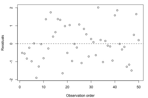
The plot is used to detect non-independence. The plot is only appropriate if you know the order in which the data were collected. In the plot, y-axis is residuals and x-axis is time (or other indicators for ordering). Here is a plot suggesting non-independence (i.e., residuals bounce randomly around the residual = 0 line):

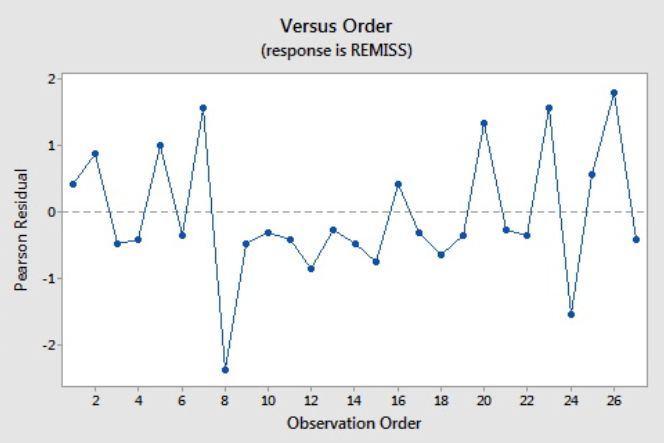
The following plot shows a time trend:

2. For Logistic Regression

2.1. Residuals

In logistic regression diagnostics, residuals also play a central role. However, the calculation of residuals in logistic regression differs from that in linear regression. Below, we introduce two commonly used residuals in logistic regression.

\begin{equation*} d_{i}=s_i\sqrt{-2\biggl(y_{i}\log({\hat{p}_{i}})+(1-y_{i})\log({1-\hat{p}_{i}})\biggr)} \end{equation*}

Deviance Residual
where $s_i=1$ if $y_i = 1$ and $s_i=-1$ if $y_i = 0$
It is the term in the log-likelihood function >>> $\sum_i d_i^2 = -2l(\hat{\beta})$

r_i =\frac{y_i-\hat{p_i}}{\sqrt{\hat{p_i}(1-\hat{p_i})}}

Pearson Residual
$y_i \sim Bern(p_i)$ >>> standardize $y_i$ : $(y_i-p_i)/\sqrt{p_i(1-p_i)}$
Thus, Pearson residual can be regarded as the standardized y using predicted p.

2.2. For Goodness-Of-Fit

1) GOF Test with Deviance

H_0: \text{Model fits data well} \\ H_1: \text{Saturated Model}

Test statistic: Deviance
- Deviance is defined as the difference of log-likelihoods between the fitted model and the saturated model: $D = 2(l_{saturated\ model}-l_{your\ model})$ .
- For grouped data, saturated model is the model that predicts $\hat{p}_i = \sum_{\in \mathbf{x}_i} y_i/n_{\mathbf{x}_i}$ ; for ungrouped data, the log-likelihood of the saturated model is exactly 0.
- Data in either grouped or ungrouped format produce the same fitted model and, therefore, the same log-likelihood for the fitted model. However, the saturated models differ in the two cases, leading to different deviances.
- Hence, GOF test using deviance only applies on Grouped Data because deviances computed from ungrouped data do not have an approximate chi-squared distribution. Moreover, even if the grouped data, when the group size $n_i$ ’s are small, the chi-square approximation is very bad so that we cannot rely on the testing result.
- Remark: The difference in deviances can be reliably used for a likelihood ratio test to compare models, regardless of whether the data is grouped or ungrouped.
- In r, it is called “residual deviance.”
Null distribution: chi-squared distribution with df = △(#ofParameters)
- The number of parameters in the saturated model = number of rows in the grouped data (i.e., unique $\mathbf{x}_i$ ).
2) GOF Test with Pearson’s Chi-Squared statistic
Same H0 and H1.
Different test statistic.
Same null distribution.

3) GOF Test with Hosmer & Lemeshow statistic

Ungrouped data that can be grouped >>> transform into grouped format >>> do GOF
Ungrouped data that cannot be grouped, maybe due to having continuous predictors >>> use this method, which is also a chi-squared test.

2.3. Residual Plotting

Some say that residual plots are nearly useless when $n_i$ s are small or using ungrouped data (source), while others say that in this case residual plots are still useful (source).

Pearson residuals/Deviance residuals vs. Index

Should randomly bounce within ±3 (or more strict, ±2)
Horizontal band centered around 0 >>> constant variance due to standardization
Similar: Pearson residuals/Deviance residuals vs. Predicted values $\hat{\beta}^Tx_i$

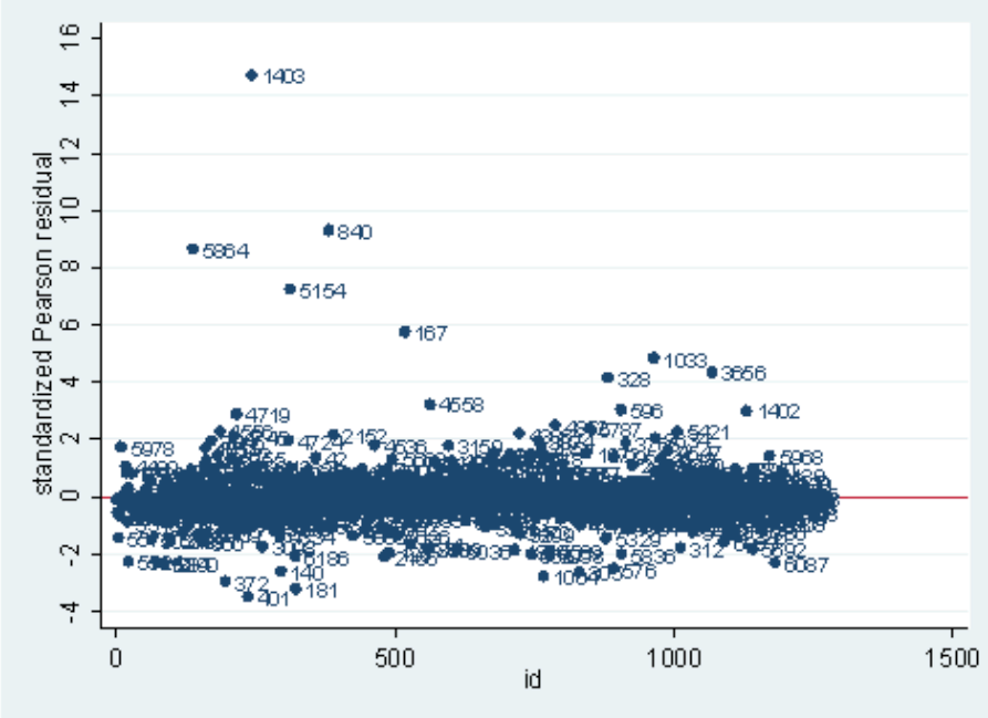
In this plot, we can identify some outliers. For example, index=1403 has a very high Pearson residual.
There are also logistic-regression-adapted version of leverage values and Cook’s distance. The physical meanings are the same.