Method | Structural Equation Models

The note is based on the contents of the introduction to SEM in R.

Table of contents

• 1. Basic concepts
  • 1.1 Terms
  • 1.2 Path diagram
• 2. Model without latent variables
  • 2.1 Simple regression (1 ex & 1 en)
  • 2.2 Multiple regression (2+ ex & 1 en)
  • 2.3 Multivariate regression (2+ ex & 2+ en)
  • 2.4 Path analysis (Multivariate reg & en ~ en)
• 3. Model with latent variables
  • 3.1 Measurement model (factor analysis)
  • 3.2 Structural Model
• 4. Model evaluation: model fit index
  • 4.1 Model chi-square
  • 4.2 CFI (Comparative Fit Index)
  • 4.3 TLI (Tucker Lewis Index)
  • 4.4 RMSEA

1. Basic concepts

Structural equation modeling (SEM) is an umbrella term referring to a framework of linear models designed to explore relationships among both observable and unobservable variables.

1.1 Terms

• Observed vs. Latent:
  • Observed variable: exists in the data (i.e. item/manifest variable)
  • Latent variable: does not exist in the data (i.e. construct)
• Exogenous vs. Endogenous:
  • Exogenous variable: not be explained by the model (like IV)
  • Endogenous variable: be explained by the model (like DV)
• Indicator, factor, loading (terms in factor analysis):
  • Indicator: an observed variable (i.e. item)
  • Factor: an latent variable defined by indicators
  • Loading: the path between an indicator and a factor

1.2 Path diagram

The following example is a structural model with two measurement models. Both exogenous variable (i.e. independent variable) and endogenous variable (i.e. dependent variable) are latent variables, which means that they are not derived directly from the data. Instead, they are constructed from some observable indicators respectively.

2. Model without latent variables

All exogenous and endogenous variables are observed.

2.1 Simple regression (1 ex & 1 en)

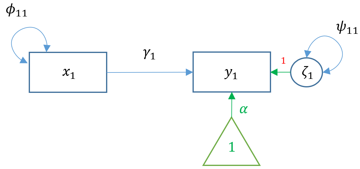
m1 = '
    # regression
      read ~ 1 + motiv
    # variance (optional)
      motiv ~~ motiv
'
m1 = sem(m1, data=dat)
print(summary(m1))

Regressions:
                Estimate  Std.Err  z-value  P(>|z|)
read ~
    motiv          0.530    0.038   13.975    0.000

Intercepts:
                Estimate  Std.Err  z-value  P(>|z|)
.read             -0.000    0.379   -0.000    1.000
 motiv             0.000    0.447    0.000    1.000

Variances:
                Estimate  Std.Err  z-value  P(>|z|)
 motiv            99.800    6.312   15.811    0.000
.read             71.766    4.539   15.811    0.000

• Intercepts:
  • .read: intercept
  • motiv: motiv’s variance
• Variances:
  • .read: residual variance
  • motiv: motiv’s mean
• Note: lavaan uses MLE to do estimating; lm uses OLS instead.

2.2 Multiple regression (2+ ex & 1 en)

m2 = '
    # regression
      read ~ 1 + ppsych + motiv
    # covariance
      ppsych ~~ motiv
'
m2 = sem(m2, data=dat)
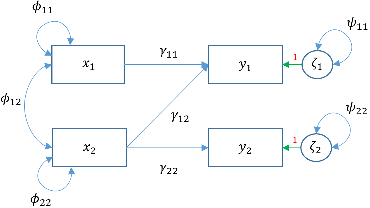
print(summary(m2))

2.3 Multivariate regression (2+ ex & 2+ en)

Modeling multiple endogenous variables simultaneously:

m3a = '
    # regressions
      read  ~ 1 + ppsych + motiv
      arith ~ 1 + motiv
    # covariance
    # (lavaan estimates the covariance between endogenous variables by default)
      ppsych ~~ motiv
'
m3a = sem(m3a, data=dat)
print(summary(m3a))

Regressions:
                Estimate  Std.Err  z-value  P(>|z|)
   read ~
     ppsych       -0.216    0.030   -7.289    0.000
     motiv         0.476    0.037   12.918    0.000
   arith ~
     motiv         0.600    0.036   16.771    0.000

Covariances:
                Estimate  Std.Err  z-value  P(>|z|)
  ppsych ~~
    motiv        -24.950    4.601   -5.423    0.000
 .read ~~
   .arith         39.179    3.373   11.615    0.000

Intercepts:
                Estimate  Std.Err  z-value  P(>|z|)
   .read          -0.000    0.361   -0.000    1.000
   .arith         -0.000    0.357   -0.000    1.000
    ppsych        -0.000    0.447   -0.000    1.000
    motiv          0.000    0.447    0.000    1.000

Variances:
                Estimate  Std.Err  z-value  P(>|z|)
   .read          65.032    4.113   15.811    0.000
   .arith         63.872    4.040   15.811    0.000
    ppsych        99.800    6.312   15.811    0.000
    motiv         99.800    6.312   15.811    0.000

Turn off the estimation of covariance between endogenous variables:

m3d = '
    # regression
      read  ~ 1 + ppsych + motiv
      arith ~ 1 + motiv
    # covariance
      ppsych ~~ motiv
      read   ~~ 0 * arith
'

The above two models are not saturated models because the reports from lavaan show that there are remaining degrees of freedom (i.e. df ≠ 0): df(m3a)=1, df(m3d)=2. Add all possible parameters about endogenous variables to make the model saturated - df(m3e)=0:

m3e = '
  # regression
    read  ~ 1 + ppsych + motiv
    arith ~ 1 + ppsych + motiv
  # covariance
    ppsych ~~ motiv
'

2.4 Path analysis (Multivariate reg & en ~ en)

Multivariate regression is a special case of path analysis, which allows an endogenous variable to be explained by other endogenous variables:

m4a = '
  # regression
    read  ~ 1 + ppsych + motiv
    arith ~ 1 + motiv + read
  # covariance
    ppsych ~~ motiv
'

This model is not saturated with a df=1, which means you have left room to work with for adding parameters to make your model more complex. modindices function helps you decide add what:

print(modindices(m4a, sort=TRUE))

     lhs op    rhs    mi    epc sepc.lv sepc.all sepc.nox
20  arith  ~ ppsych 4.847  0.068   0.068    0.068    0.068
17  arith ~~ ppsych 4.847  6.368   6.368    0.100    0.100
22 ppsych  ~  arith 4.847  0.158   0.158    0.158    0.158
25  motiv  ~  arith 4.847  0.632   0.632    0.632    0.632
14   read ~~  arith 4.847 16.034  16.034    0.314    0.314
19   read  ~  arith 4.847  0.398   0.398    0.398    0.398
18  arith ~~  motiv 4.847 25.472  25.472    0.402    0.402

mi is called 1-degree chi-square statistic, which means the model chi-square will drop how much after adding the term. However, be careful to change the model specification unless you have enough evidence from theories.

3. Model with latent variables

3.1 Measurement model (factor analysis)

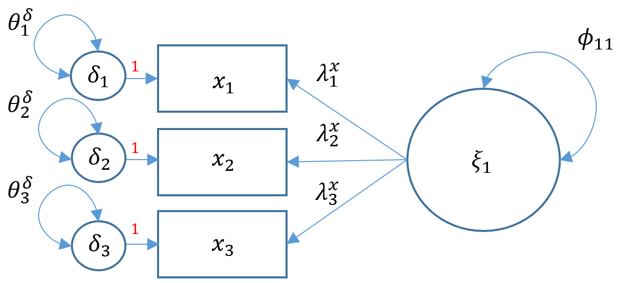
m5a = '
  # indicator equation: factor =~ indicators
    risk =~ verbal + ses + ppsych
  # intercepts (by default no intercepts)
    verbal ~ 1
    ses    ~ 1
    ppsych ~ 1
'
m5a = sem(m5a, data=dat)
print(summary(m5a, standardized=TRUE) )

lavaan 0.6.17 ended normally after 37 iterations

Estimator                                         ML
Optimization method                           NLMINB
Number of model parameters                         9

Number of observations                           500

Model Test User Model:

Test statistic                                 0.000
Degrees of freedom                                 0

Parameter Estimates:

Standard errors                             Standard
Information                                 Expected
Information saturated (h1) model          Structured

Latent Variables:
                Estimate  Std.Err  z-value  P(>|z|)   Std.lv  Std.all
risk =~
    verbal         1.000                               6.166    0.617
    ses            1.050    0.126    8.358    0.000    6.474    0.648
    ppsych        -1.050    0.126   -8.358    0.000   -6.474   -0.648

Intercepts:
                Estimate  Std.Err  z-value  P(>|z|)   Std.lv  Std.all
.verbal            0.000    0.447    0.000    1.000    0.000    0.000
.ses              -0.000    0.447   -0.000    1.000   -0.000   -0.000
.ppsych           -0.000    0.447   -0.000    1.000   -0.000   -0.000

Variances:
                Estimate  Std.Err  z-value  P(>|z|)   Std.lv  Std.all
.verbal           61.781    5.810   10.634    0.000   61.781    0.619
.ses              57.884    5.989    9.664    0.000   57.884    0.580
.ppsych           57.884    5.989    9.664    0.000   57.884    0.580
 risk             38.019    6.562    5.794    0.000    1.000    1.000

• In order to identify a factor model with three or more items:
  • marker method fixes the first loading of each factor to 1.
  • variance standardization method fixes the variance of each factor to 1 but freely estimates all loadings.
• By default, lavaan reports the results of the marker method (1.000, 1.050, -1.050); by requesting the standardized version, lavaan reports the results of the variance standardization method in Std.all column (0.617, 0.648, -0.648).

3.2 Structural Model

Two steps:

• First, construct measurement models.
• Second, specify how the latent variables relate to each other.

This is a structural model with two endogenous variables (i.e. a mediation analysis model):

m6b = '
  # measurement models
    adjust  =~ motiv + harm + stabi
    risk    =~ verbal + ses + ppsych
    achieve =~ read + arith + spell
  # regression
    adjust ~ risk
    achieve ~ adjust + risk
'
m6b = sem(m6b, data=dat)
print(summary(m6b, standardized=TRUE, fit.measures=TRUE))

4. Model evaluation: model fit index

In regression analysis, there are four common criteria for evaluating a model: 1) adjusted R2; 2) MSE(mean square error); 3) RSE(residual standard error); and 4) information criterion(AIC & BIC). In SEM, there are also four commonly used indexes for model evaluation. Here are some important points to remember:

• The model fit indexes only have true meanings when the model’s degree of freedom is greater than 0 (i.e. not a saturated model).
• The model fit indexes are test statistics with a null hypothesis stating, the model fits the data well. Specifically, this null hypothesis implies that the model-implied covariance matrix $\Sigma(\theta)$ is identical to the population covariance matrix $\Sigma$.
• Hence, rejecting the null hypothesis means that our model does not fit the data well.

Request lavaan for additional fit statistics:

summary(model, fit.measures=TRUE)

4.1 Model chi-square

• The chi-square value increases when there is a larger difference between the current model-implied covariance matrix $\Sigma(\hat{\theta})$ and the sample covariance matrix $S$ - more probable to reject H0.
• When Model Test User Model: P-value (Chi-square) < 0.05, reject H0.
• 👎 Drawback: the chi-square is extremely sensitive under large samples. You may always get a significant p-value when sample size is greater than 400. In this case, you should refer to other indexes.

4.2 CFI (Comparative Fit Index)

It is a relative fit index - comparing your model with the saturated model based on a baseline model (just like the test of goodness of fit in logistic regression - see more details):

“An relative fit index assesses the ratio of the deviation of the user model from the worst fitting model (a.k.a. the baseline model) against the deviation of the saturated model from the baseline model.”

• The closer the CFI is to 1, the better the fit of the model.
• Empirically, CFI greater than 0.90 (or 0.95) indicates a good fit.

4.3 TLI (Tucker Lewis Index)

It is also a relative fit index:

• The closer the TLI is to 1, the better the fit of the model.
• Empirically, TLI greater than 0.90 indicates a good fit.
• TLI and CFI are highly correlated so only one of the two should be reported.

4.4 RMSEA

It is not a relative fit index. Instead, it is a absolute index which does not involve comparisons. Some rules of thumb:

• $\le 0.05$ → good fit
• $>0.05$ but $<0.08$ → reasonbale fit
• $\ge 0.1$ → poor fit