Method | Instrument Variables

1. Motivation and insights
2. Univariate case
3. Multivariate case
4. Two-Stage Least Square(2SLS)
5. References

1. Motivation and insights

First, we may not always have panel data available to address endogeneity and the fixed effects model cannot manage omitted variables that change both across entities and over time. Second, endogeneity due to reverse causality cannot be addressed simply by controlling variables. Therefore, we need to use other methods like the instrumental variable method.

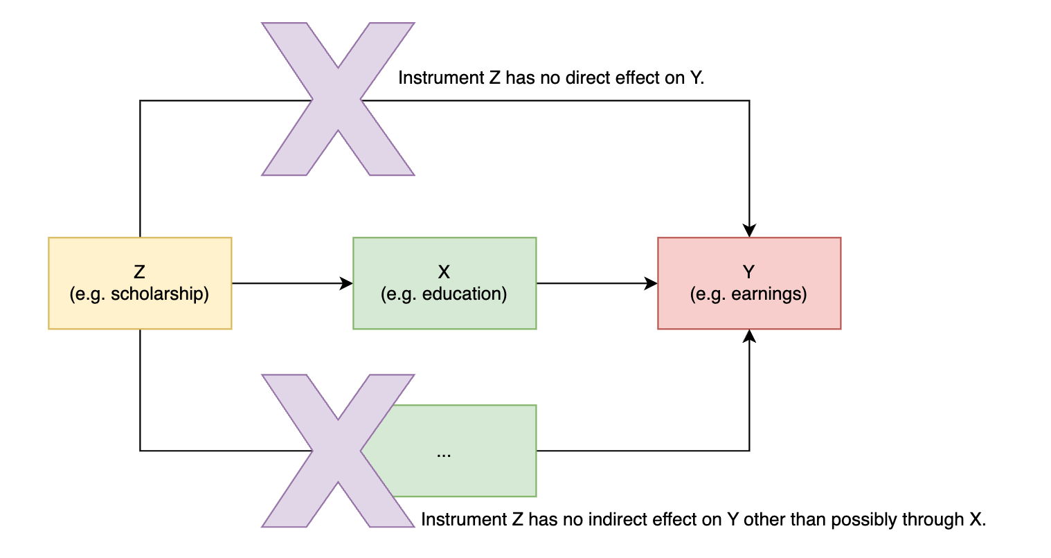
The insight behind the IV method is quite straightforward: If we find a variable Z that has a direct effect on X but not on Y, and does not indirectly affect Y through other paths, then if we observe an total effect of Z on Y, that effect can only be caused by X. Thus, it can be concluded that X affects Y.

In this case, we refer to Z as an instrument for X to identify the causal effect from X to Y. In summary, a good instrument should satisfy at least three conditions: 1) It affects the endogenous variable X; 2) It is (as good as) randomly assigned so that its association with Y can be interpreted as the causal effect; 3) It has no direct effect or other indirect effects on Y.

A not-so-good IV: Doctors are randomly selected to receive advice to remind their patients that it is flu season and they should take a flu shot, can we use it as an instrument for taking the flu shot, so we can estimate the impact of taking the flu shot on sick days? In this case, the IV may violate the condition 3: Doctors often provide additional advice when reminding people to get vaccinated, such as drinking more orange juice during flu season and washing hands frequently. These suggestions may influence behaviors like drinking orange juice and handwashing, ultimately making people less likely to get sick, rather than solely through the pathway of vaccination. In such cases, using such IV would attribute the effects of these alternative pathways solely to vaccination, introducing bias.

2. Univariate case

Our population model:

y = \beta_0 + \beta_1 x + u

where $Cov(x,u) \ne 0$ , indicating there is an endogeneity problem. If there is a variable z that satisfies the following two conditions:

Cov(z,u) = 0\\Cov(z,x) \ne 0

Then the variable z is called an instrumental variable for variable x. The first condition above is referred to as instrumental exogeneity, and the second condition is referred to as instrument relevance:

Instrumental exogeneity cannot be statistically verified; instead, it must be argued on a case-by-case basis.
Instrumental relevance can be verified by conducting an auxiliary regression x~z and check the significance of the coefficient.
(The assumption of randomly-assigned IV does not appear in Wooldridge’s textbook.)

Using the instrumental variable z can help us in identifying β1:

\begin{align*}Cov(z,y) &= Cov(z, \beta_0 + \beta_1 x + u)\\&= \beta_1Cov(z, x) + Cov(z, u)\\&= \beta_1Cov(z, x)\end{align*}

Hence:

\beta_1 = \frac{Cov(z,y)}{Cov(z,x)}

Then, we can use the sample to obtain the IV estimation of β1:

\hat{\beta_1}^{IV} = \frac{\sum_i(z_i-\bar{z})(y_i - \bar{y})}{\sum_i(z_i-\bar{z})(x_i - \bar{x})}

Remarks:

Instrumental variable estimators are consistent but biased, hence it is preferable not to use them under small sample conditions.
The derivation of standard errors for IV estimators is omitted here. However, it’s important to note that their standard errors are often larger than those of OLS estimators, which is a cost of this method.
When the covariance between z and x is small but not zero, using such weak instruments for estimation often yields poor results.

3. Multivariate case

Consider following model with two independent variables y2 and z1:

y_1 = \beta_0 + \beta_1y_2 + \beta_2 z_1 + u_1

where y2 is endogenous and z1 is exogenous:

Cov(y_2,u_1) \ne 0\\Cov(z_1,u_1) = 0

Now we want to find an IV for y2. Pay attention: z1 cannot be used as the IV for y2 even though it may be correlated with y2 because z1 is already one of the independent variables in the regression equation. We need another IV for y2.

Assume there is a variable z2, such that:

Cov(z_2, u_1) = 0\\Cov(z_2, y_2) \ne 0

In this case, we have three equations for Moments Estimation(矩估计) :

E(u_1) = 0\\E(z_1u_1) = 0\\E(z_2u_1) = 0\\

We can use the sample to solve for three estimators: $\hat{\beta_0}, \hat{\beta_1}, \hat{\beta_2}$ - called IV estimators. Besides, we have to check the instrument relevance in the presence of z1 (i.e. y2~z1+z2):

y_2 = \pi_0 + \pi_1z_1 + \pi_2z_2 + v_2

We have to test $\pi_2 \ne 0$ in this model.

4. Two-Stage Least Square(2SLS)

In the aforementioned case, we have only one IV (i.e. z2) for y2, the endogenous regressor. If we have another exogenous variable z3 which is also correlated with y2 and uncorrelated with u1, then both z2 and z3 can serve as instrumental variables for y2.

Here comes a question: which one is the best IV for y2? The answer is none of them. The best IV should be the linear combination of them. It can be easily proven that the linear combination of IVs is also an IV. Besides, we can also add z1 to the linear combination since z1 is also an exogenous variable. We first estimate y2~z1+z2+z3 and obtain the fitted value as the IV (need to test whether $\pi_2 \ne 0$ or $\pi_3 \ne 0$ ):

\hat{y}_2 = \hat{\pi}_0 + \hat{\pi}_1z_1 + \hat{\pi}_2z_2 + \hat{\pi}_3z_3

After getting the new IV, we can use a two-stage regression approach by regressing $y_1 \sim \hat{y}_2 + z_1$ to obtain OLS estimates. This estimate is equivalent to the IV estimate obtained through the method of moments. To sum up,

[Stage 1] The endogenous variable ~ all exogenous variables
- Check the significance of the exogenous variables that are not original covariates
- Obtain the fitted values for the endogenous variable
[Stage 2] Replace the endogenous variable in the original regression equation with the fitted values, then conduct regression again to obtain IV estimates.

5. References

Wooldridge, J. M. (2013). Introductory Econometrics : a Modern approach. (5th ed.). Mason Cengage Learning.
Lecture 21: Endogeneity and Instrument Variables - YouTube
ivreg: Two-Stage Least-Squares Regression with Diagnostics